Math 121 - Calculus for Biology I Spring Semester, 2004 More Applications of Nonlinear Dynamical Systems
	© 2001, All Rights Reserved, SDSU & Joseph M. Mahaffy San Diego State University -- This page last updated 19-Mar-04

More Applications of Nonlinear Dynamical Systems

1. Sockeye Salmon Populations
2. Ricker's Model
3. Analysis of the Ricker's Model
4. Simulation of Ricker's Model
5. Sockeye Salmon of Skeena River Revisited
6. Worked Examples
7. Hassell's Model
8. Study of a Beetle Population
9. Analysis of Hassell's Model
10. Beetle Study Revisited
11. References

The previous section on the discrete logistic growth model established the key elements for studying the qualitative behavior of a discrete dynamical model. First, the equilibria for the model are found, then using the derivative of the updating function, the local stability of the equilibria are determined. This section extends our analysis to other nonlinear discrete dynamical models, which in certain cases improves on the discrete logistic growth model. The study of the stability of these models uses a variety of the differentiation techniques learned earlier.

The first extension to the study of the Malthusian growth model was the logistic growth model, which improved on the Malthusian growth model by accounting for the crowding effects that result in natural limits to populations. The logistic growth model employs a quadratic updating function, which becomes negative for large populations. Ecologists have modified the logistic growth model in several ways to make the updating function more realistic and better able to handle largely fluctuating populations. One model that is often used in fishery management is Ricker's model. Populations of insects undergo large fluctuations, so again the logistic growth with its negative updating function for large populations is replaced with an alternative model, Hassell's model. Below these models are fit to data, then analyzed using the techniques learned in the previous sections.

Sockeye Salmon Populations

Recently, the salmon population in the Pacific Northwest has become sufficiently endangered that many salmon spawning runs could become extinct. (This already happened years ago in California.) Salmon are unique in that they breed in very specific fresh water lakes and die. Their offspring migrate a tortuous path to the ocean, where they mature for about 4-5 years. Then an unknown urge causes the mature salmon to migrate at the same time to return to the exact same lake or river bed where they hatched 4-5 years earlier. The adult salmon breed and die with their bodies providing many essential nutrients that nourish the stream where their young will repeat this process. Human activity from damming rivers, forestry, which allows the water to become too warm, and agriculture, which results in runoff pollution, all adversely affect this complex life cycle of the salmon. Many of the ancient salmon runs have now gone extinct.

This life cycle of the salmon is a clear example of a complex discrete dynamical system. Because of the importance of this fish to many people in the Pacific Northwest, there have been many studies of the salmon populations. Below is a table listing four year averages of the sockeye salmon (Oncorhynchus nerka) in the Skeena river system in British Columbia from 1908 to 1952. (The Canadian river systems have not been as severely affected by other human activities as the ones in the U.S., but rapid development in their forests are likely to have similar effects.) The table lists the four year averages from the starting year of the data being averaged. Since it is 4 and 5 year old salmon that spawn, each grouping of 4 years is a rough approximation of the offspring of the previous 4 year average of salmon. (It is complicated because the salmon have adapted to have either 4 or 5 year old mature adults spawn, but this will be ignored in our modeling efforts.)

Four Year Averages of Skeena River Sockeye Salmon

We want to use these data to create a discrete dynamical system to describe the population of salmon in the Skeena river watershed. This system can be analyzed to determine information about expected salmon runs to study the health of the ecosystem.

Ricker's Model

The logistic growth model extends the Malthusian growth model and includes an additional term for the crowding effects on population growth. As populations become more crowded, the resource limitations result in a decrease in the population growth rate. The logistic growth model was given by

where P_n is the population at the n^th time period, r is the Malthusian growth rate, and M is the carrying capacity of the population. Our section on the logistic growth model showed that this model did a reasonable job for predicting certain yeast populations. This model can be applied reasonably well to unicellular organisms that are provided a fixed amount of nutrient, such as a culture of yeast growing in a controlled environment. However, this model does not fit the data for many organisms, such as the salmon population listed above. If a population experiences large fluctuations, then for very large populations the logistic growth model may return a negative population in the next generation, which is clearly unrealistic. Several alternative models have been proposed, where the updating function remains positive.

One such model is Ricker's model, which it is claimed was originally formulated using studies of salmon populations. This model is very frequently used in fisheries management problems. We will apply this model to the sockeye salmon data listed above.

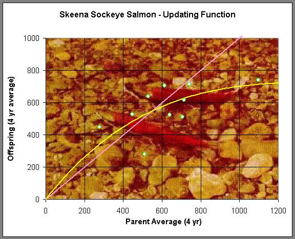
Ricker's model is given by the equation

where a and b are positive constants that are fit to the data. Below is a graph showing the data of successive generations from the averaged data listed above. For example, the parent population of 1908-1911 is averaged to 1,098,000 salmon/year returning to the Skeena river watershed, and it is assumed that the resultant offspring that return to spawn from this group occurs between 1912 and 1915, which averages 740,000 salmon/year. This produces the furthest point on the right in the graph below.

(Picture is from the Canadian Fishing Co.)

A nonlinear least squares fit of the Ricker function above is used on the data and the best Ricker's model for the Skeena sockeye salmon population from 1908-1952 is given by

P_n+1 = R(P_n) = 1.535P_nexp(-0.000783P_n).

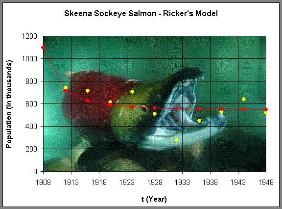
Before we analyze this model, we simulate the model using the initial average in 1908 as our starting point and see how well the model traces the data above. Below is a graph of this simulation.

(Picture is from GBarkman Art and Design.)

We see that the Ricker's model has the population leveling off at a stable equilibrium around 550,000, which is relatively consistent with the data. There are a few fluctuations, which is what we would expect from the variations in the environment. However, the model suggests that this is a robust ecological system that maintains a healthy population. Below we will perform a more detailed analysis of this model and use the techniques that we have developed in earlier sections to find equilibria, graph the Ricker's function, and determine the stability of the Ricker's model.

Analysis of the Ricker's Model

As in the logistic model, Ricker's model has two equilibria with one of them being the trivial or zero equilibrium. The equilibria for this model are found by setting P_e = P_n+1 = P_n, which gives

From this equation, we readily see that

P_e = 0 and

P_e = ln(a)/b.

Note that the second equilibrium is positive (real for our model) only if a > 1.

The previous section notes that the stability of the equilibria are related to the derivative of the updating function evaluated at the equilibrium. Thus, for Ricker's model, the stability condition for the equilibria is given by

Thus, we need to be able to take the derivative of the Ricker's updating function, which requires the product rule of differentiation. Applying the product rule to the Ricker's function R(P) = aPe^-bP gives

The equilibrium P_e = 0 is stable if R '(0) = a < 1, while if R '(0) = a > 1, then the solution monotonically grows away from this equilibrium. At the equilibrium P_e = ln(a)/b, the derivative of the Ricker's updating is

R '(ln(a)/b) = a e^-ln(a)(1 - ln(a)) = 1 - ln(a).

Recall that a > 1 for a positive equilibrium. From the stability results of the previous section, the analysis of the Ricker's model in general is as follows:

1. The solution of Ricker's model is stable and monotonically approaches the equilibrium P_e = ln(a)/b provided a < e = 2.7183.
2. The solution of Ricker's model is stable and oscillates as it approaches the equilibrium P_e = ln(a)/b provided e < a < e² = 7.389.
3. The solution of Ricker's model is unstable and oscillates as it grows away from the equilibrium P_e = ln(a)/b provided a > e² = 7.389.

There are several Worked Examples that illustrate this qualitative analysis of Ricker's model.

Sockeye Salmon of Skeena River Revisited

From the notes above we have that the best Ricker's model for the Skeena sockeye salmon population from 1908-1952 is

P_n+1 = R(P_n) = 1.535P_nexp(-0.000783P_n).

We find the equilibria and stability of the equilibria for this particular case. Let P_e = P_n+1 = P_n, then

Thus, the two equilibria are P_e = ₀ and _547.3 with the latter equilibrium value close to the value observed in the graph of the simulation above.

Next we differentiate R(P) and see that

Thus, at _{Pe = 0},

R'(0) = 1.535 > 1,

which shows that the equilibrium at 0 is unstable as expected. At P_e = _547.3,

R'(547.3) = 1.535e-0.4285(1 - 0.4285) = 0.571 < 1,

which implies that this equilibrium is stable with solutions monotonically approaching the equilibrium, as we observed in the simulation.

Hassell's Model

As noted above, Hassell's model, which is written in the form of a quotient, is an alternative to the Logistic growth model and Ricker's model and is frequently applied to insect populations. Hassell's model for studying the dynamics of insect populations has the form:

 

where a, b, and c are parameters that are chosen to match the data for a population study of some insect. The numerator of H(P_n) is the Malthusian growth model, so that at low population densities, the population grows exponentially. (Recall that this requires a > 1.) As the population increases, the denominator increases, which slows the rate of growth. The denominator is a composite function, including a linear function, 1 + bP_n, which is raised to the c power. Thus, differentiation of H(P_n) requires the chain rule.

Study of a Beetle Population

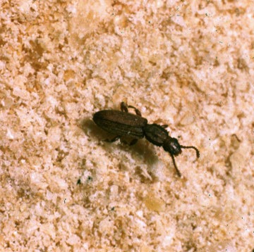
In 1946, A. C. Crombie [1] studied several beetle populations to try to better understand their dynamics under the strict control of a constant amount of food regularly supplied. He maintained the amount of food at 10 grams of cracked wheat added weekly, then regularly took census of the beetle populations. These experimental conditions match the assumptions used by the Logistic growth model. One study was on Oryzaephilus surinamensis, the saw-tooth grain beetle. Below is a table of his data (with some minor modifications to fill in times of uncollected data and an initial one week shift).

By plotting the data of P_n+1 vs. P_n, we can fit an updating function to the data, then use this updating function to study the population dynamics with an appropriate discrete dynamical model. This section compares Hassell's model to the Logistic growth model. Below is a graph showing the best fit to Crombie's data for Oryzaephilus surinamensis for both Hassell's model and the Logistic growth model. (The best fit for Hassell's model was found using the fminsearch routine in MatLab, while the Logistic growth model used Trendline in Excel.)

 

With 3 parameters, Hassell's updating function is capable of fitting the data better than the quadratic function of the Logistic growth model. Hassell's updating function has the added advantage that it never becomes negative, which was a property of Ricker's model. The best model from Hassell's formula is given by:

 

while the best Logistic growth model satisfies

 

With the updating functions above, these discrete dynamical models are simulated and compared to the data of A. C. Crombie. Below shows the simulations of the models with the data (assuming the models agree with the data at week 0). We note that an alternative method of fitting the models is to apply the least squares best fit to the simulation rather than finding the best fitting updating function. When this technique is applied the simulations are very close, but again Hassell's model fits better.

We can readily see that Hassell's model does appear to simulate the data better, especially having the early rapid rise in the population. All seem to tend toward a similar carrying capacity. For more details on the behavior of these models, we perform our standard analysis of the discrete models, locating equilibria and using the derivative to test the local behavior of these models.  

Analysis of Hassell's Model

We return to the general Hassell's model to obtain the equilibria and determine stability conditions for the equilibria. Following the usual techniques for studying discrete dynamical models, the equilibria of Hassell's model are found by letting P_e = P_n = P_n+1. Thus, we solve

This is equivalent to

One of the equilibria is P_e = 0, while the other solves (1 + bP_e)^c = a. This latter equation is easily solved by taking the c^th root of each side, then completing the algebra, so

Note that the this equilibrium requires the condition a > 1.

To determine the stability of the equilibria, we differentiate the function H(P). This requires the quotient rule, which in turn requires differentiating the denominator, which is a composite function. Below we use the chain rule to differentiate the term in the denominator.

Now applying the quotient rule, we find that

This formula shows that H '(0) = a, but since a > 1 for a positive equilibrium to exist, this condition implies that the zero (or trivial) equilibrium in unstable with solutions monotonically growing away from this equilibrium. At the other equilibrium, we can evaluate H '(P_e) and obtain

This calculation shows that the stability of the carrying capacity equilibrium is very dependent on both a and c, but not b. Further algebra on the derivative calculation above and stability results of the previous section give the following general stability results for Hassell's model for c > 2:

1. The solution of Hassell's model is stable and monotonically approaches the equilibrium P_e = (a^1/c - 1)/b provided 1 < a < (c/(c - 1))^c.
2. The solution of Hassell's model is stable and oscillates as it approaches the equilibrium P_e = (a^1/c - 1)/b provided (c/(c - 1))^c < a < (c/(c - 2))^c.
3. The solution of Hassell's model is unstable and oscillates as it grows away from the equilibrium P_e = (a^1/c - 1)/b provided a > (c/(c - 2))^c.

This result can be readily modified to handle the cases where 1 < c < 2 or 0 < c < 1, but these cases are left to the reader.

Beetle Study Revisited

When we apply the qualitative analysis results from the logistic growth section or the material above, then we can provide more information about the models described above. The best Logistic growth model that fits the Crombie data is given by

 

while the best Hassell's model for the saw-tooth grain beetle satisfies

 

For the logistic growth model, the carrying capacity is the non-zero solution to

P_e = 1.962P_e - 0.002189P_e²

0.002189P_e = 0.962

P_e = 439

which gives M = 439. The derivative evaluated at this equilibrium is

L'(439) = 1.962 - 0.004378(439) = 0.04 < 1.

Thus, our stability results show that the logistic growth model predicts that populations of Oryzaephilus surinamensis will grow monotonically and level off at the equilibrium P_e = 439.

For Hassell's model, the positive equilibrium is

P_e = 3.255P_e/(1 + 0.0073P_e)^0.8178.

(1 + 0.0073P_e)^0.8178 = 3.255

P_e = (3.255^1.223 - 1)/0.0073 = 443

which gives a carrying capacity of M = 443. The derivative evaluated at this equilibrium is

H '(443) = (0.8178/3.255^1.223) + (1 - 0.8178) = 0.375 < 1.

Thus, this stability result shows that Hassell's model predicts that populations of the saw-tooth grain beetle will grow monotonically and level off at the equilibrium P_e = 443. The logistic and Hassell's growth models have similar carrying capacities with the same qualitative behavior of monotonically approaching this equilibrium. These qualitative behaviors are easily seen in the simulation graphically shown above. Our studies above show that functions that look quite different can result in very similar behavior.

References:

[1] A. C. Crombie (1946) On competition between different species of graminivorous insects, Proc. R. Soc. (B), 132, 362-395.

[2] Ricker, W.E. 1958. Handbook of computations for biological statistics of fish populations. Fisheries Research Board of Canada.

[3] Shepard, M. P. and Withler, F. C. (1958) Spawning stock size and resultant production for Skeena Sockeye. J. Fisheries Research Board of Canada 15: 1007-1025.

[4] Walters, C.J. 1986. Adaptive management of renewable resources. Macmillan (NY).

[5] Walters, C.J. and Hilborn, R. 1968. Ecological optimization and adaptive management. Annual Rev. of Ecology and Systematics 9, 157-188.