Hassell's Model Alternate Fit

We analyzed the data of A. C. Crombie (1946) for the population dynamics of Oryzaephilus surinamensis, the saw-tooth grain beetle. Our analysis before concentrated on the updating function, and we found the least squares best fit to the data for the updating function. The time-series simulations did not fit the actual data very well, especially the logistic growth model.

This appendix uses the nonlinear least squares best fit of the model simulations directly to the Crombie data. The Logistic growth model is given by

P_n+1 = P_n + rP_n(1 - P_n /M),

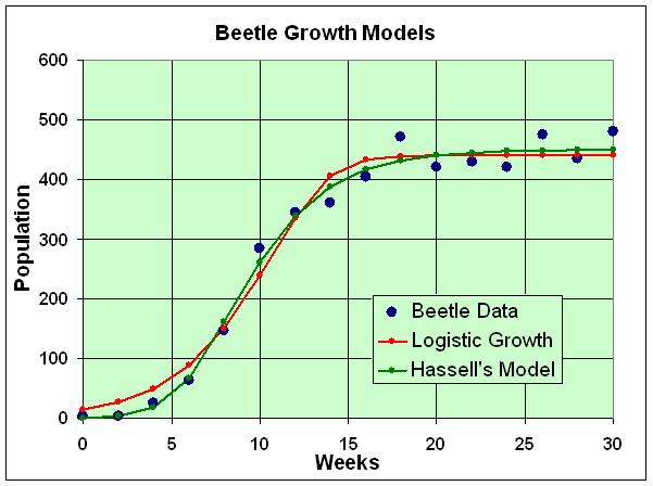
where P₀ is the initial population, r is the Malthusian growth rate, and M is the carrying capacity of the population. These 3 parameters are varied to minimized the sum of square errors between the model and the data. (See graph below.) The minimum sum of square error is 11,745. The best fitting parameters are P₀ = 14.62, r = 0.8847, and M = 440.3. Thus, the logistic growth model that best fits Crombie's data is

From our work on the logistic growth model, the carrying capacity for this model is M = 440.3.

The general form for Hassell's model is given by

which has the 3 parameters a, b, and c along with the initial condition P₀. When a nonlinear least squares is performed with this model, the minimum sum of square error is 6478, significantly better than the logistic growth model above. The best fitting parameters are P₀ = 0.6063, a = 5.799, b = 0.07479, and c = 0.4959. (See graph below.) Thus, the Hassell's growth model that best fits Crombie's data is

From our equilibrium analysis before, this model has a carrying capacity of

M = (a^1/c - 1)/b = 449.6,

which is similar to the prediction of the logistic growth model.

This least squares analysis gives similar values for the parameters for the logistic growth model as compared to our analysis where the updating function is fit to the data, but very different ones for Hassell's growth model, indicating less robustness for Hassell's model. Below is a graph showing the data and the two models. Both models track the data well, but Hassell's has a better fit, especially in the earlier weeks. The extra parameter in Hassell's model is one reason that the curve fits the data better. The qualitative behavior of these two models is essentially the same. Clearly, the parameter fits performed here are superior to ones used for the updating function, but either method can be employed depending on the desired outcome.