SDSU


Math 121 - Calculus for Biology I
Spring Semester, 2004
Logistic Growth - Worked Examples

 © 2001, All Rights Reserved, SDSU & Joseph M. Mahaffy
San Diego State University -- This page last updated 18-Mar-04


Logistic Growth - Worked Examples

  1. Analysis of the Logistic Growth Model
  2. Growth Rate for Logistic Model
  3. Examples for Stability of the Logistic Growth Model
  4. Stability of the Malthusian Growth Model
  5. Logistic Growth with Emigration
  6. Logistic Growth Model Applied to the U.S. Population


These examples expand on the qualitative techniques for analyzing the logistic growth model


Examples for Analysis of the Logistic Growth Model

Example 1:

Consider the discrete logistic growth model

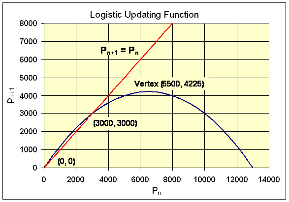
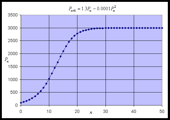
Pn+1 = f1(Pn) = 1.3Pn - 0.0001Pn2.


Solution:

For equilibria, substitute Pe for Pn and Pn+1 into the discrete logistic growth model

Pe = 1.3Pe - 0.0001Pe2

0 = 0.3Pe - 0.0001Pe2 = Pe (0.3 - 0.0001Pe)

Pe = 0 and

0.3 - 0.0001Pe = 0 or Pe = 3000


  • Compute the derivative of f1(Pe)

f1'(P) = 1.3 - 0.0002P.

  • At Pe = 0

f1'(0) = 1.3 > 1

  • The solution monotonically grows away from this equilibrium, as expected


  • At Pe = 3000

f1'(3000) = 1.3 - 0.6 = 0.7 < 1

  • The discrete logistic model monotonically approach this equilibrium
  • This equilibrium is said to be stable


Example 2: Modify the example above and consider the discrete logistic growth model

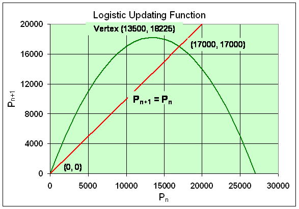
Pn+1 = f2(Pn) = 2.7Pn - 0.0001Pn2.


  • Find all the equilibria for this model
  • Determine the behavior of the solution near these equilibria
  • Sketch a graph of the updating function and the identity map Pn+1 = Pn


Solution: Substitute Pe for Pn and Pn+1 into the discrete logistic growth model

Pe = 2.7Pe - 0.0001Pe2

0 = 1.7Pe - 0.0001Pe2 = Pe (1.7 - 0.0001Pe)

Pe = 0

Pe = 17000


  • The derivative is

f2'(P) = 2.7 - 0.0002P

  • At Pe = 0, the derivative is

f2'(0) = 2.7 > 1

  • The solution monotonically grows away from this equilibrium


  • At Pe = 17000, the derivative is

f2'(17000) = 2.7 - 3.4 = -0.7

  • Since -1 < f2'(17000) < 0, the discrete logistic model oscillates and approaches this equilibrium
  • This equilibrium is also stable


  • To graph the updating function, find the P-intercepts and the vertex
    • The P-intercepts are 0 and 27,000
    • The vertex is at (13500, 18225)
  • Below is the graph with the identity function and significant points shown on the graph


Simulation of this model with an initial value of P0 = 100 and 20 iterations
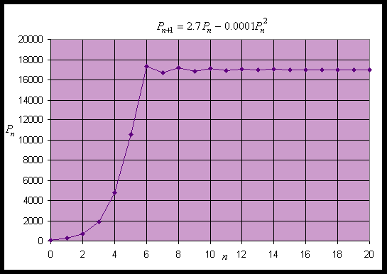


Example 3: Another change in the discrete logistic growth model gives

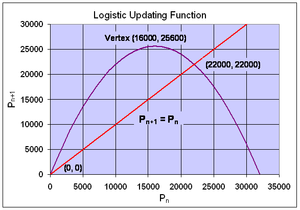
Pn+1 = f3(Pn) = 3.2Pn - 0.0001Pn2


  • Find all the equilibria for this model
  • Determine the behavior of the solution near these equilibria
  • Sketch a graph of the updating function and the identity map Pn+1 = Pn


Solution: Substitute Pe for Pn and Pn+1 into the discrete logistic growth model

Pe = 3.2Pe - 0.0001Pe2

0 = 2.2Pe - 0.0001Pe2 = Pe (2.2 - 0.0001Pe)

Pe = 0

Pe = 22000


  • The derivative satisfies

f3'(P) = 3.2 - 0.0002P

  • At Pe = 0, the derivative is

f3'(0) = 3.2 > 1

  • Tthe solution monotonically grows away from Pe = 0


  • At Pe = 22000, the derivative is

f3'(22000) = 3.2 - 4.4 = -1.2

  • Since f2'(17000) < -1, the discrete logistic model oscillates and moves away from this equilibrium
  • This equilibrium is unstable


  • To graph the updating function, find the P-intercepts and the vertex
    • The P-intercepts are 0 and 32,000
    • The vertex is at (16000, 25600)
  • Below is the graph with the identity function and significant points shown on the graph


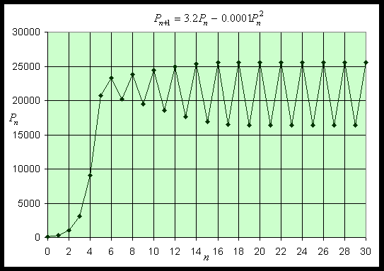
  • Simulation of this model with an initial value of P0 = 100 and 30 iterations
    • The simulation shows the solution growing away from Pe = 0
    • It settles into a period 2 oscillation taking on the values 16417 and 25583


Example 4 (Growth Rate Function for Logistic Model):

  • An alternate way to look at discrete population growth models is to consider the population at the (n+1)st generation as being equal to the population at the nth generation plus the growth of the population, g(pn), between the generations
  • Consider the logistic growth model given by the equation
pn+1 = pn + g(pn) = pn + 0.05 pn (1 - 0.0001pn),

where n is measured in hours

  • The equilibria can be readily found by determining when the growth rate is zero.

a. Assume that p0 = 500 and find the population for the next three hours, p1, p2, and p3.

b. Find the p-intercepts and the vertex for

g(p) = 0.05 p(1 - 0.0001p)

Sketch a graph of g(p).

c. By finding when the growth rate is zero, determine all equilibria for this model and find the stability of the equilibria.


Solution:

a. The first three iterations are

p1 = p0 + g(p0) = 500 + 0.05(500)(1 - 0.0001(500)) = 524,

p2 = 524 + 0.05(524)(1 - 0.0001(524)) = 549,

p3 = 549 + 0.05(549)(1 - 0.0001(549)) = 574.


b. The p-intercepts are found by solving

g(p) = 0.05 p(1 - 0.0001p) = 0,

Thus,

p = 0 or

p = 10,000.

p = 5,000

g(5000) = 0.05(5000)(1 - 0.0001(5000)) = 125
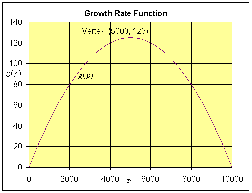


c. From the graph above, it is clear that the growth rate is zero at 0 and 10,000, so the equilibria occur at

pe = 0 and 10,000.


pn+1 = f(pn) = 1.05 pn - 0.00005pn2.

f '(pn) = 1.05 - 0.0001pn.


Example 5 (Stability of the Malthusian Growth Model):

  • The discrete Malthusian growth model has a solution that grows exponentially
  • Show that the only equilibrium of the Malthusian growth model is unstable


Solution:

  • Assume that there is a positive growth rate, so r > 0
  • The general Malthusian growth model is

Pn+1 = (1 + r)Pn

  • The equilibrium with Pe for Pn and Pn+1 satisfies

Pe = (1 + r)Pe

rPe = 0 or Pe = 0


  • The only equilibrium for the discrete Malthusian growth model is the trivial solution, Pe = 0
  • The derivative of the right hand side of the model is (1 + r), which is greater than one
  • Any positive growth rate implies that the discrete Malthusian growth model is unstable
  • The solution monotonically moves away from the equilibrium
  • This agrees with the exponential growing behavior shown earlier


Example 6 (Logistic Growth with Emigration):

g(p) = 0.71 p - 0.001p2 - 7.


The discrete dynamical model for this population model is

pn+1 = pn + g(pn) = pn + 0.71 pn - 0.001pn2 - 7,

where n is measured in generations.

a. Assume that p0 = 100 and find the population for the next three generations, p1, p2, and p3.

b. Find the p-intercepts and the vertex for g(p) and sketch a graph of g(p).

c. By finding when the growth rate is zero, determine all equilibria for this model.


Solution:

a. The next three generations are

p1 = p0 + g(p0) = 100 + 0.71(100) - 0.001(100)2 - 7 = 154,

p2 = 154 + 0.71(154) - 0.001(154)2 - 7 = 233,

p3 = 233 + 0.71(233) - 0.001(233)2 - 7 = 337.


b. The growth function satisfies

g(p) = 0.71 p - 0.001p2 - 7

g(p) = -0.001(p2 - 710p + 7000)

g(p) = -0.001(p - 10)(p - 700).


The p-intercepts satisfy g(p) = 0, so

p = 10 or p = 700.


The vertex occurs halfway between the p-intercepts, so p = 355 and

g(355) = -0.001(345)(-345) = 119.

The maximum growth occurs when the population is 355 with a maximum growth of 119 individuals/generation.


The graph of g(p) is shown below showing the p-intercepts at p = 10 and 700 and the vertex.
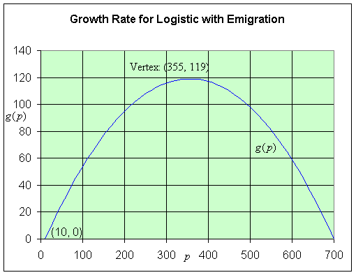
c. From the graph above, it is clear that the growth rate is zero at p = 10 and 700, so the equilibria occur at pe = 10 and 700.


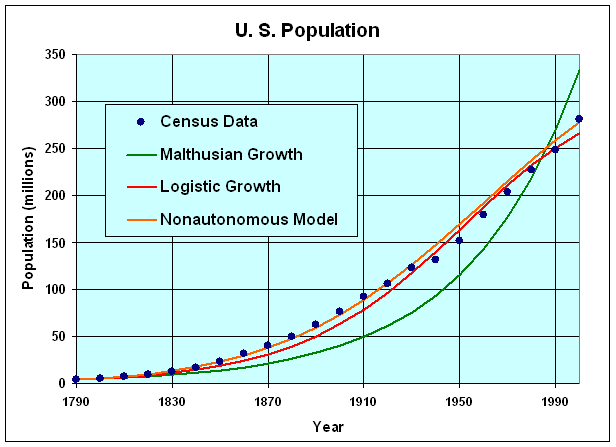
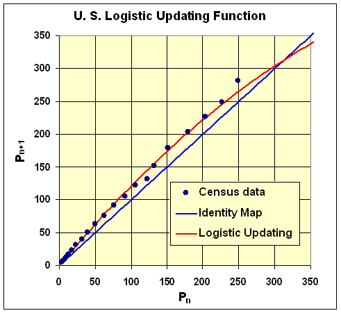
Example 7 (U. S. Census with Logistic Growth Model)


Pn+1 = 1.2354 Pn.


Pn+1 = (1.3835 - 0.0155n)Pn.


F '(P) = 1.3064 - 0.00195P.