1. Growth of Brewer's Yeast
2. Logistic Growth Model
3. Bernoulli's Method 
4. Fitting the Logistic Growth Model
   1. Algebraic Fit to the Yeast Data
   2. Least Squares Fit to the Yeast Data
5. Return to Qualitative Behavior of Differential Equations
6. References

This section uses Bernoulli's method to solve the Logistic Growth model. The derivation of this model is found in the section that begins our study of the qualitative behavior of differential equations. This section begins with a classic example of growth of Saccharomyces cerevisiae. The experiment was designed to satisfy the conditions of logistic growth. Extensions of this experiment are used later in these lecture notes to show the interaction of two species competing for resources. This section ends showing two techniques to match the data of the experiments on Saccharomyces cerevisiae.

Growth of Brewer's Yeast

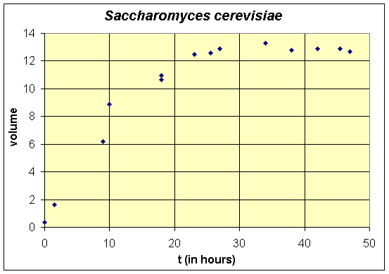
G. F. Gause [1] ran a series of experiments that validated the logistic growth equation for a collection of microorganisms. His experiments were designed to study the growth of one or two species of yeast and other unicellular organisms growing in an environment with a limited source of nutrient. The two species study is analyzed in lecture notes on the qualitative analysis of systems of two differential equations. One of the species that was studied was brewer's yeast, Saccharomyces cerevisiae. Below we present a table and graph combining two experiments that used identical conditions for growing the culture of yeast. We will use two methods to fit these data to the logistic growth model. The experimental data is shifted by 6 hours from the original, since an initial yeast volume is not presented. (Experimentally, Gause grew the cultures to carrying capacity, then transferred "two drops" of culture to start his experiment. His earliest data point was 6 hours later, which is given below as time zero.) Note that the volume of the yeast was used as a measurement of its growth and the units were defined by markings on a 3.5 mm diameter centrifuge tube, so are not particularly well defined.

These experiments illustrate a problem when the experimentation does not use the feedback (shown in the introduction to the lectures). The experiments are meant to verify the logistic growth model, yet they were not redesigned after testing against the mathematical model. These experiments lack the very important initial values, which we will see are very important, and there are a paucity of data through the primary growth phase of the yeast. This leads to large margins of error in the choice of some of the parameters. However, the experiment does provide good data for the carrying capacity of the yeast under Gause's experimental design. An estimate of the carrying capacity is readily found by averaging the data points after growth of the yeast has leveled off. We can see that the growth has leveled off after about 24 hours, so if we average these data points, we obtain

Thus, the carrying capacity is about 12.9, which matches well with the value of 13.0 reported by Gause. The next part of these notes examines the solution of the logistic growth equation, then further below we find the other growth parameters for this experiment using two methods.

Logistic Growth Model

In the notes for Math 121, we saw that the discrete logistic growth model is an improvement over the discrete Malthusian growth model because of the additional term that accounts for crowding of the population. This model was shown to work quite well for a yeast population and in the Labs for different populations of beetles. One major problem with the discrete logistic growth model is that it has no explicit solution. Furthermore, there are examples of the discrete logistic growth model that become chaotic in behavior.

In the section beginning our study of the qualitative behavior of differential equations, the continuous logistic growth model was derived from the discrete logistic growth model and is given by the following:

In this section, we show one method for solving this differential equation. The continuous logistic growth model is clearly a separable differential equation, but separating variables leaves you with an integral that requires a technique of integration called partial fraction decomposition and then still requires a messy amount of algebra. (Clearly, you could use integral tables or Maple to solve the integral.) This example is usually analyzed using this separation of variables method for students in Calculus and Differential Equation books.

Bernoulli's Method

However, there is a simpler method for solving this problem developed by Jakob Bernoulli in the late 1600's. This is simply another substitution technique (which has been the topic of study in many of our previous sections) that reduces the problem to a linear problem. Consider the logistic growth model with the substitution

If we differentiate this substitution, then the chain rule gives

Let us multiply the logistic growth model by - P ^-2. The resulting equation is

or

This is converted into our variable z(t), and gives the differential equation

or

Notice that the last form of the differential equation in z(t) is basically the same problem that we encountered when solving the differential equations for Newton's law of cooling or pollution in a lake. Thus, we want another substitution, say w(t) = z(t) - 1/M. Note that z(0) = 1/P₀, so w(0) = 1/P₀ - 1/M. Thus, we are solving the initial value problem

This has the solution

so

However, P(t) = z ^-1(t), so with a little algebra, we can write the solution of the logistic growth model as

Example: Consider the logistic growth model describing the growth of a bacteria given by the equation

Solve this differential equation and graph its solution for 0 < t < 200. What is the carrying capacity for this culture of bacteria? Determine how long until the population reaches half of its carrying capacity.

Solution: Our solution of this problem follows the techniques described above. We begin by making a substitution of

Differentiation and the chain rule gives

We multiply our example by - P ^-2, and the resulting equation is

which is equivalent to the differential equation (through substitution) in the variable z(t) given by

From the initial condition on P(t), this substitution also gives the initial condition

As noted above, the differential equation for z(t) is just like our Newton's Law of cooling problems, so we make a further substitution of

Note that w(0) = z(0) - 1/2000 = 0.01-0.0005 = 0.0095. Thus, we want to solve the initial value problem

This has the solution

so

However, since P(t) = z ^-1(t), it follows that

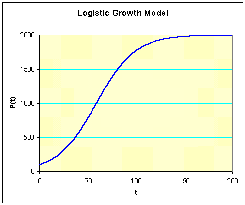
Note that this is exactly the solution you obtain by substituting r =0.05, M =2000, and P₀ = 100 into the general solution given above this example. The graph of this solution is presented below.

The carrying capacity for this population of bacteria can be found in two ways. From the solution, we know that as t becomes large, the exponential function, e^-0.05t, approaches zero. It follows that the population, P(t), approaches 2000 for large t. Alternately, we simply examine the differential equation and realize that the carrying capacity is the parameter, M, and M = 2000.

The time at which the population reaches half the carrying capacity is the time where P(t) = M/2 = 1000. Thus, we solve

Rearranging the equation on the right, then taking the logarithm of both sides, we have

Thus, the time to reach half the carrying capacity satisfies

which can be seen in the graph above.

Fitting the Logistic Growth Model - Yeast 

The best technique to fit the experimental data uses a nonlinear least squares method as we have done before in the computer lab. Details of this technique and a link to an Excel spreadsheet for computing the least squares best fit model are presented below. However, nonlinear least squares methods need some reasonable initial estimate before they are likely to converge. We begin by showing how to use an algebraic method to fit the data reasonably well. This algebraic solution is used with Excel's nonlinear solver routine to obtain the best model fit for the experimental data above.

Algebraic Fit to the Yeast Data

The solution to the logistic growth equation is given by the formula

Thus, we need to determine the values of the parameters P₀, M, and r. The experimental design included special efforts to control the initial innoculation of the growing cultures of yeast, thus minimizing the variation of the volume of the initial culture of yeast. This allows us to assume that P₀ is known. From the original article by Gause [2], we are not given that the initial volume of yeast cells innoculated into the experimental culture, so we adjusted the time by 6 hours. Thus, our initial data as seen in the table at the beginning of this section is

(Recall that this is a volume measured on the centrifuge tube.) The experiment was designed to satisfy the assumptions of the logistic growth model, so a limited supply of nutrient was provided in regular (3 hr) intervals. Gause found that after 24 hours, his culture of Saccharomyces cerevisiae leveled off at the carrying capacity of the population for the amount of nutrient that he provided. This allows us to use the experimental data to estimate the carrying capacity of this population. The average of the data after 24 hours is given above and gives us the parameter

(Again we note that Gause used 13.0 for his value of M, but had no justification.) It follows that the design of the experiment gives easy access to the parameters P₀ and M (though as noted early in this section, the experiment would have benefitted from data collected immediately following innoculation).

It only remains to estimate the growth rate of the culture, r. This parameter is estimated by examining the data and selecting a data point that is representative of the expected S-shaped logistic curve seen above. Typically, you select one of the data points that is close to half the carrying capacity to give the best results. Since the data were a combination of two experiments and our initial value comes from the first experiment, it follows that the accuracy is probably better if we also take the second choice from the data of this first experiment. We selected the volume of the yeast population at t = 9 hr, which had P(9) = 6.2 (volume units of yeast), which is roughly half of the carrying capacity. With this information substituted into the solution of the logistic growth model shown above, we can solve for the remaining parameter r. Thus, we must solve the equation

Cross multiplying, we have

By taking logarithms, we have 9r = ln(31.34), so

which is substantially higher than the r = 0.21827 reported by Gause. This makes our initial estimate for a model to this yeast growth as

The model reported by Gause [2] is

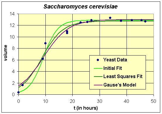
Below we will show this model, Gause's reported model, and the least squares best fit model that is presented in the next subsection.

Least Squares Fit to the Yeast Data

The computations above provide a reasonable fit to the data. However, we can use the power of the computer to obtain what is considered the best fit to the data using a nonlinear least squares technique. The technique requires a good initial estimate, which is provided by the calculation above. A discussion of the fitting of data using a nonlinear least squares best fit can be found in lecture notes for Math 121 with several examples provided in the computer labs earlier this semester (for example the Fourier series fit to the lynx and hare data), where more details are available on how to construct an Excel spreadsheet for this analysis.

An Excel spreadsheet can be downloaded to view how to best fit a logistic growth model to the data in the table at the beginning of this section. The method of finding this "best" model to fit the data is computed by minimizing the expression given by the formula

There are 14 data points with the volume of yeast at the different times (t_i) are denoted P_d(t_i). The model depends on the three parameters P₀, M, and r. The model volume of yeast given by the solution of the logistic growth equation with the three values inserted (starting with the values computed above, P₀ = 0.37, M = 12.9, r = 0.3828) at each of the times for the data points is subtracted from the value of the data at these times. This gives the error between the model and the data for a given set of parameters. Each of these error values is squared, and the sum of the squared errors is computed. Next Excel's Solver routine that can be found under the Tools heading is using to minimize this sum of squares error. (If the reader downloads the Excel spreadsheet, then the parameter values are found in the cells H2-H4 and the sum of square errors is in cell E17. The data are in columns B and C, while the model simulations are found in columns K-M.) The least squares best fit to the data, which is found by Excel gives the parameter values

which gives the best fit model to the yeast data as

This minimization process is very computationally intensive! Note that this model differs from the model presented by Gause in the literature. Most likely, Gause fixed the values of P₀ and M, then only minimized r, which can be done with a simple Newton's method. Recall that he did not have powerful computers in the early 1930s, so this was his most reasonable approach to finding a best fit model.

Below we graph the solutions presented above

All three models provide reasonable estimates to the data. We see that our initial model, which was found using algebraic techniques, nicely fits the first two points of the first experiment in the data and matches the carrying capacity fairly well. However, its growth rate does appear to be a little too high and its initial value seems too low. The carrying capacities of all three models are very close, which is what we would expect from the qualitative behavior analysis. There is a fair discrepancy in the growth rates, which as noted above is largely due to the fact that there needed to be more data points acquired in the experiments during the primary growth period. This is where experimenters and modelers need to develop better communication links to improve both the models and the experimental design.

References

[1] G. F. Gause, Struggle for Existence, Hafner, New York, 1934.

[2] G. F. Gause (1932), Experimental studies on the struggle for existence. I. Mixed populations of two species of yeast, J. Exp. Biol. 9, p. 389.