Math 121 - Calculus for Biology I Fall Semester, 2003 Discrete Malthusian Growth
	© 2001, All Rights Reserved, SDSU & Joseph M. Mahaffy San Diego State University -- This page last updated 14-Oct-03

Discrete Malthusian Growth

Outline of Chapter

1. Population of the United States
2. Discrete Malthusian Growth
3. Applet for U. S. Population Growth
4. Example of Malthusian Growth
5. Worked Examples
6. Improved Malthusian Growth Model
7. References

This section begins the dynamical modeling part of the course. The discrete dynamical system developed in this section examines snapshots of a population at specific time intervals. Later Calculus extends the discrete Malthusian growth model to all times.

Population of the United States

The United States takes a census of its population every 10 years. (This last year saw the census taken again and results are just now coming out, while the interpretation of those results will be argued for several years.) The census has important ramifications for many aspects of our society, such as budgeting federal payments and representation in Congress. The method of taking the census and how it is analyzed has been a very hot issue pitting the Republicans against the Democrats in 1999 with the issue landing in the Supreme Court. The Republicans wanted a strict interpretation of the Constitution, knowing that a direct head count always undercounts minorities and the poor, who vote predominantly Democratic. The Democrats claimed that the Constitution framers wanted an accurate count of the populace, so that modern statistical methods should be employed. This would naturally give them an advantage in the voting. (The Supreme Court came down in the middle pleasing neither party and saying that the Constitution requires a head count, which will be used for allocating Congressional seats and districting, while the more accurate statistical count may be used for apportioning the money for Federal funding.) The arguing over the numbers will go on for several years as each group tries to use the numbers to their best advantage to gain federal money and political power. Despite the political controversy over the numbers, accurately predicting these demographic data are important for planning our communities in the future. At the base of all calculations for the future population predictions is some type of mathematical model. Current models are quite sophisticated, but first we must appreciate the basic models behind them. Below we present the census data for the history of the U. S.

The growth rate between each decade can be determined by dividing the census at one date by the census a decade earlier and subtracting one. The calculation below shows how to compute the growth rate for the decade of 1790-1800.

Thus, the growth rate for this decade is 35.1%. The javascript below performs this computation to give the growth rate for any decade in the history of the U. S.

From the javascript above, we find that the growth rates for decades following 1790, 1800, and 1810 are 35.1%, 36.4%, and 33.1%, respectively, which averages 34.9% per decade. This growth rate remains almost constant until 1860, so this information should allow us to estimate the census data up until 1860 using a model with a constant growth.

The simplest mathematical model says that the population in the next decade is equal to the current population plus the current population times the average growth rate, r, of the population. The model begins with some starting population, say in 1790. The future populations are predicted at each decade (discrete time intervals) by starting with this initial given population, then finding the next population from the previous population by multiplying by (1 + r). This gives a sequence of predicted populations each based solely on the population from the preceding decade. For example, using the population of 3,929,214 in 1790, we would multiply by 1.349 to get an estimate of the population in 1800. Mathematically, we have

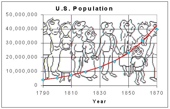
Notice that this prediction is less than 8,000 off the actual census value or a 0.15% error. We could repeat this process to predict each of the succeeding census populations up until 1860 (a period where the growth rate remains fairly constant). Thus, the population in 1840 would be projected to be 1.349 times the population predicted in 1830. Below we provide a table showing this type of constant growth model applied to the census up until 1870.

Notice that the error remains small until 1870 because of the fairly constant rate of growth. Most of the predicted populations are a little high, especially in 1870, suggesting that throughout the 19^th century the growth rate declined. The declining growth rate is a general trend that we observe for the U. S. and is something that will be accounted for in an improved model developed later in this section.

Between 1860 and 1870, the Civil War occurred, which is one cause of the dramatic decline in the rate of growth of the population in the U. S. Thus, the 1870 prediction is one that you would expect to be poor. In fact, the shift from the primarily agricultural society to the industrial revolution is more significant in causing the decline in the rate of growth. We will study more about crowding effects in the next lecture section.

Below is a graph of the population model and the data from the table above.

Discrete Malthusian Growth

Let the integer n represent the number of decades after 1790 and define P_n to be the population for the n^th decade after 1790 (with P₀ again representing the population in 1790). The population for one decade is estimated by using the population from the previous decade and adding to it the average percent growth multiplied by the population from the previous decade. The mathematical model based on this description is given by:

where r is the average growth rate. Our calculations above suggest that we use r = 0.349 to estimate the population of the U. S. from 1790 to 1860.

This equation is the Discrete Malthusian Growth model (named after the work of Thomas Malthus (1766-1834)). The Discrete Malthusian Growth model is a special example of Discrete Dynamical systems or Difference equations, which we will study in more detail as the semester progresses. Population models using difference equations are commonly used in Ecological modeling as one can often determine the population of a species or collection of species knowing the population of the previous generation of the species being studied. The Malthusian growth model states that the population of the next generation is simply proportional to the population in the current generation, which is what is written in the equation above.

Solution of Discrete Malthusian Growth Model

There are not many discrete models that have an explicit solution. However, it is easy to solve the discrete Malthusian growth model. From the model above, we see that

Thus, the general solution of this model is given by

This shows why Malthusian growth is also known as exponential growth. The solution to the model that is given by the equation above is an exponential function with a base of 1+ r and power n representing the number of iterations after the initial population is given.

Applet for Malthusian Growth for the U. S. population

There is nothing special about starting the Malthusian growth model at the first census point in 1790. The Malthusian growth model assumes a constant growth rate, so is unlikely to do well predicting the population over long periods of time where growth rate varies. Because of the exponential nature of the Malthusian growth model, this model can rapidly diverge from the actual population. Below is an applet where you can vary the starting time, ending time, and growth rate to see how the Malthusian growth model works for the U. S. census data.

 sourcecode for growth6g

If you choose the interval from 1790 to 1860 with a growth rate of r = 0.349, then the Malthusian growth model matches quite well. However, if you try to fit the entire range of data from 1790 to 1990, then you will find no value of r that allows the Malthusian growth model to fit the data. (Using the average growth rate of 23.5% has the Malthusian growth model match the data at 1790 and 1990, but fails to do well for the intermediate data points.) By making r into a function which depends on either time or population or both, then we can see how this model can be improved. For more information on human population growth you might want to visit the UN website on population.

Example of Malthusian Growth

Let us suppose that a population of yeast, satisfying Malthusian growth, grows 10% in an hour. If the population begins with 100,000 yeast, then find the population at the end of 4 hours. How long does it take for this population to double?

Solution:

The population of yeast satisfies the equation

The population after one hour is P₁ = 1.1P₀ = 110,000. After two hours, P₂ = 1.1P₁ = (1.1)²P₀ = 121,000. Thus, after 4 hours,

For the population to double, it must reach 2P₀ = 200,000. Thus, we must solve

By taking the logarithms of both sides we have

A hyperlinked page is provided to give more Worked Examples for Malthusian Growth.

Improved Malthusian Growth Model

The section above presents a discrete Malthusian Growth model based on the U. S. population from census data. In this section, we extend the Malthusian Growth model to include time varying reproduction rates. We will compare the two models on how they do in predicting the 2000 census, which is the last of the data points presented.

The average growth rate over the first few decades gives a growth rate that is much too high for population prediction in the 20^th century, which suggests that the simple Malthusian Growth model above with some average growth rate is likely to over predict the 2000 census. This section compares the discrete Malthusian growth model using the average growth rate over all the data and an improved modified model that uses a time dependent growth rate, which is acquired by fitting a straight line through the growth rate data. (Recall our earlier studies of using a least squares best fit to data.)

The general discrete dynamical population model is given by

where f is a function depending only on the population P at time t_n. This difference equation is said to be autonomous as it does not have a temporal or time dependence. A more general difference equation is given by

which is a nonautonomous difference equation.

The growth rate for the Malthusian Growth model is computed by dividing the population at one census date by the population at the previous census date. When the average is taken over all the census dates from 1790 to 1990 in the table above, we find that the average growth rate

This results in the discrete Malthusian growth model

Clearly, this growth rate is too low for the early years, and too high for later years. If we use this model to predict the population in the year 2000 starting with the population in 1790, then from the solution of the Malthusian Growth model above we have that the year 2000 is 21 decades after 1790, so with P₀ = 3,929,214, then

This prediction is clearly too high (about 16% too high).

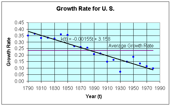
A modified time dependent growth rate can be found by fitting a line through the data from 1790 to 1990. The best fit to these growth rate data, along with the average growth rate, is seen in the graph below:

The best fit to the growth rate data from 1790 to 1990 is given by the equation

where t is the date of the census.

The resulting modified nonautonomous difference equation is given by

where t_n = 1790 + 10n and n is the number of decades after 1790. Thus, we have the model

P_n+1 = (1.3835 - 0.0155n)P_n .

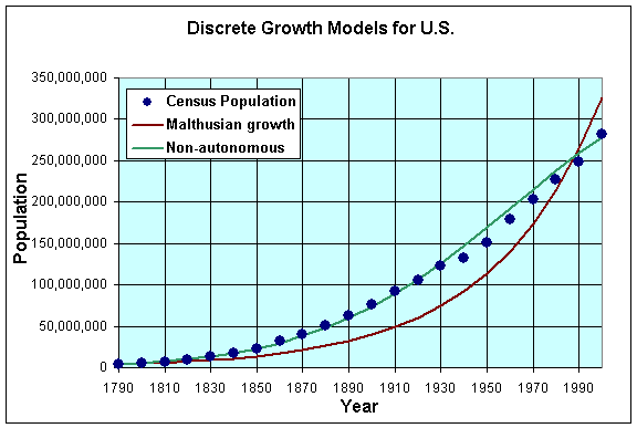
The graph below gives a comparative study of these two models. The Malthusian Growth model performs poorly as noted above because the growth rate varies too much over the time interval being considered. The Nonautonomous Discrete Malthusian Growth model matches the data quite well though runs a bit high after the severely depressed population growth during the Great Depression. Clearly, this is the better model to predict the 2000 census. 

It should be noted that computing the population using the Nonautonomous Malthusian Growth model is more complicated than the simpler Discrete Malthusian Growth model. We have the general solution for the simpler model as shown by the computation above where obtaining the population in 2000 requires only knowing the population in 1790, then raising 1.2342 to the 21^st power.

The computation for the Nonautonomous Malthusian Growth model requires finding the solution at each decade to proceed to the next decade. Thus, the model starts with the population in 1790 (= 3,929,214), then (1 + k(1790)) is computed (=1.3835) and multiplied by the population in 1790 (=3,929,214) to give the population for 1800 (= 1.3835 x 3,929,214 = 5,436,068). This is repeated. (For the second decade, the predicted population in 1800 (= 5,436,068 ) is multiplied by the computed value for 1 + k(1800) (=1.3680), to arrive at the new prediction for the population of 1810 (= 1.3680 x 5,436,068 = 7,436,540 ).)

Below is a table showing the calculations needed to get the predicted 2000 census, along with the errors as the model iterates. The second column is the actual census data, the third column calculates the factor 1 + k(t_n) = 1+ (3.158 -0.00155 t_n), where t_n is the date from the first column, needed in the Nonautonomous Malthusian Growth model, then the fourth column gives the model's prediction (P_n+1 = (1+k(t_n))P_n) and is computed by multiplying the predicted value above in the table by the factor (1 + k(t_n)) just calculated. The Error is calculated between the predicted value and the actual census data for that year.

[1] Statistical Abstracts of the United States (1993) 113 ^th ed., U. S. Department of Commerce, Bureau of the Census, Washington, DC.