Math 121 - Calculus for Biology I
Spring Semester, 2004
Logistic Growth - Worked Examples
San Diego State University -- This page last updated 17-Mar-04
|
|
Math 121 - Calculus for Biology I |
|
|---|---|---|
|
San Diego State University -- This page last updated 17-Mar-04 |
![]()
Logistic Growth - Worked Examples
This section provides a series of examples on the logistic growth model to supplement the lecture section and help understand the process on analyzing discrete dynamical equations, finding equilibria and determining the stability of the equilibria. We also include the Malthusian growth model to see how this analysis applies to this discrete dynamical model.
Examples for Analysis of the Logistic Growth Model
Example 1: Consider the discrete logistic growth model given by the equation
where n is measured in weeks.
a. Assume that P0 = 200 and find the population for the next three weeks, P1, P2, and P3.
b. Find all the equilibria for this model. Sketch a graph of the updating function (the right hand side of the equation above) along with the line Pn+1 = Pn, showing clearly on the graph the equilibria and the vertex of the parabola.
c. Use the results from the lecture section to determine the behavior of the solution near the equilibria.
Solution: a. Given P0 = 200, the updating function above generates the following populations for the next three weeks,
P1 = 1.3(200) - 0.0001(200)2 = 256,
P2 = 1.3(256) - 0.0001(256)2 = 326,
P3 = 1.3(326) - 0.0001(326)2 = 413.5.
b. To find the equilibria, we simply substitute Pe for Pn and Pn+1 into the discrete logistic growth model. This gives
The parabola has P-intercepts of 0 and 13,000, so the vertex is at (6500, 4225). Below is the graph with the identity function and significant points shown on the graph.
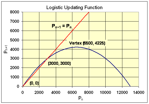
c. To determine the behavior of the model near the equilibria Pe = 0 and 3000, we need to compute the derivative of f1(Pe). This is easily done using the power rule, so
To find the behavior near Pe = 0, we compute f1'(0) = 1.3 > 1. Thus, the solution monotonically grows away from this equilibrium, which is what we expect.
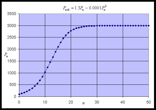
At the other equilibrium, Pe = 3000, we find f1'(3000) = 1.3 - 0.6 = 0.7 < 1. Thus, from the lecture notes, we see that solutions of the discrete logistic model monotonically approach this equilibrium. This equilibrium is said to be stable. Below we show a simulation of this model, starting with an initial value of P0 = 100 and performing 50 iterations. The simulation shows the solution growing away from Pe = 0 and approaching Pe = 3000 monotonically.
Example 2: We modify the example above slightly and consider the discrete logistic growth model given by the equation
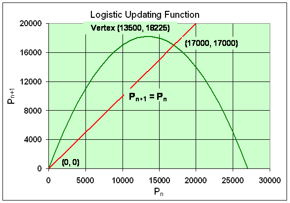
Find all the equilibria for this model and use the results from the lecture section to determine the behavior of the solution near these equilibria. Again, sketch a graph of the updating function (the right hand side of the equation above) along with the line Pn+1 = Pn, showing clearly on the graph the equilibria and the vertex of the parabola.
Solution: As in the previous example, we substitute Pe for Pn and Pn+1 into the discrete logistic growth model giving
Pe = 0 and Pe = 17000.
Below is a graph of the updating function and the identity map, showing clearly the equilibria.
The behavior of the model near the equilibria Pe = 0 and 17000 is found by computing the derivative of f2(Pe). The derivative is given by
At Pe = 0, the derivative is f2'(0) = 2.7 > 1. Thus, the solution monotonically grows away from this equilibrium.
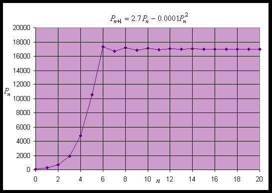
At the other equilibrium, Pe = 17000, the derivative is f2'(17000) = 2.7 - 3.4 = -0.7. Since -1 < f2'(17000) < 0, the discrete logistic model oscillates and approaches this equilibrium. This equilibrium is also stable. Below we show a simulation of this model, starting with an initial value of P0 = 100 and performing 20 iterations. The simulation shows the solution growing away from Pe = 0, then oscillates and rapidly approaches Pe = 17000.
Example 3: Another change in the discrete logistic growth model gives the equation
Find all the equilibria for this model and use the results from the lecture section to determine the behavior of the solution near these equilibria. Again, sketch a graph of the updating function (the right hand side of the equation above) along with the line Pn+1 = Pn, showing clearly on the graph the equilibria and the vertex of the parabola.
Solution: As in the previous two examples, we substitute Pe for Pn and Pn+1 into the discrete logistic growth model giving
Below is a graph of the updating function and the identity map, showing clearly the equilibria.
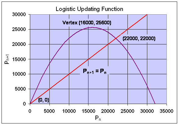
The behavior of the model near the equilibria Pe = 0 and 22000 is found by computing the derivative of f3(Pe). The derivative satisfies
At Pe = 0, the derivative is f3'(0) = 3.2 > 1. Thus, the solution monotonically grows away from Pe = 0.
At the other equilibrium, Pe = 22000, the derivative is f3'(22000) = 3.2 - 4.4 = -1.2. Since f3'(22000) < -1, the discrete logistic model oscillates and moves away from this equilibrium. Thus, this equilibrium is unstable. Below we show a simulation of this model, starting with an initial value of P0 = 100 and performing 30 iterations. The simulation shows the solution growing away from Pe = 0, then it settles into a period 2 oscillation taking on the values 16417 and 25583.
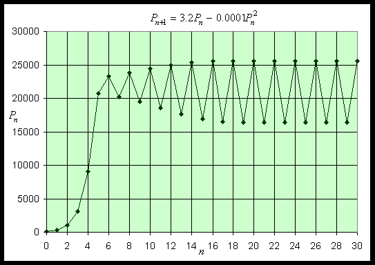
Example 4 (Growth Rate Function for Logistic Model): An alternate way to look at discrete population growth models is to consider the population at the (n+1)st generation as being equal to the population at the nth generation plus the growth of the population, g(pn), between the generations. The logistic growth model in the form of a growth function rather than an updating function is given by the equation
where n is measured in hours. The advantage of this form of the model is that equilibria occur when the growth rate is zero. Clearly when a population stops growing (growth function is zero), then it must be at an equilibrium.
a. Assume that p0 = 500 and find the population for the next three hours, p1, p2, and p3.
b. Find the p-intercepts and the vertex for
Sketch a graph of g(p).
c. By finding when the growth rate is zero, determine all equilibria for this model and find the stability of the equilibria.
Solution: a. We find the first three iterations by substituting each successive value into the given updating function. Thus,
p2 = 524 + 0.05(524)(1 - 0.0001(524)) = 549,
p3 = 549 + 0.05(549)(1 - 0.0001(549)) = 574.
b. Since g(p) = 0.05 p(1 - 0.0001p), the p-intercepts are found by solving
g(p) = 0.05 p(1 - 0.0001p) = 0,
which gives either p = 0 or 1 - 0.0001p = 0. The latter is equivalent to p = 10,000.
The vertex occurs halfway between the p-intercepts, so p = 5,000 and
g(5000) = 0.05(5000)(1 - 0.0001(5000)) = 125.
The vertex is the maximum growth rate of the population, so the maximum this population can grow is 125 individuals/hr.
The graph of g(p) is a standard parabola, which is shown below showing the p-intercepts and the vertex.
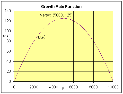
c. From the graph above, it is clear that the growth rate is zero at 0 and 10,000, so the equilibria occur at pe = 0 and 10,000. The stability is still determined by differentiating the updating function, not the growth function,
pn+1 = f(pn) = 1.05 pn - 0.00005pn2.
The derivative of the updating function is
f '(pn) = 1.05 - 0.0001pn.
At Pe = 0, the derivative is f '(0) = 1.05 > 1. Thus, the solution is unstable and monotonically grows away from Pe = 0. At the other equilibrium, Pe = 10000, the derivative is f '(10000) = 0.05. Since 0 < f '(10000) < 1, the discrete logistic model is stable and the solutions monotonically approach the equilibrium, Pe = 10000.
Example 5 (Stability of the Malthusian Growth Model):
The discrete Malthusian growth model was substantially easier to study than the logistic growth model. Its solution was simply an exponentially growing solution. Use the results from the lecture section to show that the only equilibrium of the Malthusian growth model is unstable.
Solution: We assume that there is a positive growth rate for a population of animals satisfying according to the discrete Malthusian growth model, so r > 0. The general Malthusian growth model is given by
The equilibrium is readily found by substituting Pe for Pn and Pn+1, giving
Pe = (1 + r)Pe or rPe = 0
Pe = 0.
Thus, the only equilibrium for the discrete Malthusian growth model is the trivial solution, Pe = 0. When we take the derivative of the right hand side of the model, we find that the derivative is (1 + r), which is greater than one. This means that for any positive growth rate, the discrete Malthusian growth model is unstable, and the solution monotonically moves away from the equilibrium. This is in agreement with the exponential growing behavior shown earlier.
Example 6 (Logistic Growth with Emigration): We extend the earlier example to include the possibility that the population might be affected by immigration or emigration. Suppose that the growth rate for a population is given by
This says that between each generation there is a 71% growth rate, while 0.001pn2 are lost due to crowding and 7 emigrate. The discrete dynamical model for this population model is given by
where n is measured in generations.
a. Assume that p0 = 100 and find the population for the next three generations, p1, p2, and p3.
b. Find the p-intercepts and the vertex for g(p) and sketch a graph of g(p).
c. By finding when the growth rate is zero, determine all equilibria for this model.
Solution: a. As we did in the previous example, we iterate this discrete logistic model with emigration to obtain the next three generations. Thus,
p2 = 154 + 0.71(154) - 0.001(154)2 - 7 = 233,
p3 = 233 + 0.71(233) - 0.001(233)2 - 7 = 337.
b. The growth function satisfies
g(p) = 0.71 p - 0.001p2 - 7
g(p) = -0.001(p2 - 710p + 7000)
g(p) = -0.001(p - 10)(p - 700).
The p-intercepts are found by solving g(p) = 0, which gives either
p = 10 or p = 700.
The vertex occurs halfway between the p-intercepts, so p = 355 and
g(355) = -0.001(345)(-345) = 119.
Thus, for this logistic growth model, the maximum growth occurs when the population is 355 with a maximum growth of 119 individuals/generation.
The graph of g(p) is a parabola, which is shown below showing the p-intercepts at p = 10 and 700 and the vertex.
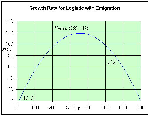
c. From the graph above, it is clear that the growth rate is zero at p = 10 and 700, so the equilibria occur at pe = 10 and 700.
Example 7 (U. S. Census with Logistic Growth Model)
The Malthusian growth model did not work well for the U. S. census data over any extended period of time because the growth rate in general has been declining for most decades in U. S. history. Can we apply the logistic growth model to the U. S. census data and get a better fit to the data and avoiding the problems of the time varying nonautonomous model developed at the end of the discrete Malthusian growth section?
The discrete Malthusian growth section included the U. S. census data from 1790 to 2000. How does one find the appropriate updating function for a logistic growth model? The best fit to a model uses the least squares best fit technique. A least squares best fit to the U. S. census data was performed to find the best Malthusian growth model and the best logistic growth model. The best Malthusian growth model is given by
Pn+1 = 1.2354 Pn.
The best logistic growth model satisfies the model

We recall that a nonautonomous model fitting the time varying growth (using a linear fit to the data) satisfied the model
Pn+1 = (1.3835 - 0.0155n)Pn.
The simulations of the Malthusian, logistic, and nonautonomous growth models are graphed below showing how well they compare to the actual U. S. census data. It is readily apparent that the Malthusian growth model does not fit the data very well, growing too slow in the early history of the U. S. and growing too rapidly more recently. The logistic growth model appears to fit the data fairly well. Still the best fit is the nonautonomous model developed in the discrete Malthusian growth section.
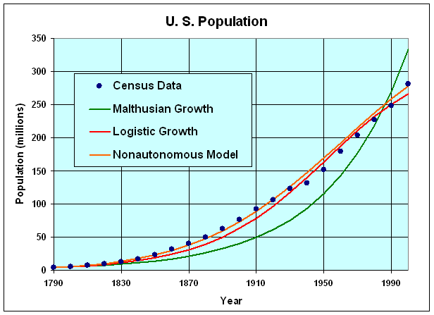
By plotting Pn+1 versus Pn, one can see how the data compares to the updating function for the logistic growth model. The graph of this updating function with the data is seen below with the identity map Pn+1 = Pn:
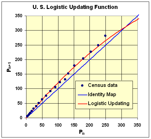
The logistic updating function very closely follows the census data except at a couple of points. We have seen that the equilibria are found by the intersection of the updating function and the identity map. The slope of the updating function at a point of intersection determines the stability of that equilibrium.
The equilibria for the logistic growth model above are Pe = 0 or 313.8 million. The derivative of the updating function is
F '(P) = 1.3064 - 0.00195P.
It follows that F '(0) = 1.3064, so Pe = 0 is unstable as expected. Similarly, F '(313.8) = 0.6936, so the equilbrium Pe = 313.8 million is stable. Thus, the logistic growth model fit to the U. S. census data predicts that the population of the U. S. will growth monotonically, then level off at 313.8 million. Note that this population is not much higher than the 2000 census value, while actual projections have the U. S. population rising to over 400 million by the middle of the next century.
The logistic growth model is easier to analyze than the nonautonomous model, but the nonautonomous model appears to fit the growth of the U. S. population better. By extending the analysis of the nonautonomous growth model, we see that the growth continues until n = 25 (actually 24.7), then this model has the population beginning to decline. Simulating this model for 25 decades (until 2040) finds that a maximum population of 318.8 million is reached. (Details of this analysis are omitted.) Note that the nonautonomous model and the logistic growth model both seem to predict a similar maximum population for the U. S., and both are unrealistically low. This shows that human populations have a more complicated dynamics than these models can predict with either time-varying or crowding factors. (Sociological and technical factors are especially difficult to incorporate into mathematical models.) Your ecology courses should help explain more details underlying the assumptions in these models, so explain a little better when the models are applicable and why they fail in other predictions. It is unlikely that human population can continue its current course, but what will be the actual scenario? Mathematical modeling can provide reasonable estimates for short term growth and allows one to predict several different possibilities for longer term growth depending on the assumptions that are entered into the model.