Outline of Chapter

1. The C period for E. coli
2. Least Squares Best Fit
3. Worked Examples
4. Juvenile Height Revisited
5. Calculating Error
6. References

In the first section we showed one of the simplest of mathematical models, which is relating one variable to another using a straight line or linear relationship. Often this is a reasonable approximation to biological data over a limited domain. This section examines the most common technique for fitting a straight line to data known as a linear least squares best fit or linear regression. (The term regression comes from a pioneer in the field of applied statistics who gave the least squares line this name because his studies indicated that the stature of sons of tall parents reverts or regresses toward the mean stature of the population.)

Finding the C period for E. coli

The bacterium Escherichia coli is capable of very rapid proliferation.(See the animated gif above to see actual E. coli growing and dividing.) Under ideal growing conditions, these bacteria can divide every 20 minutes. Its genetic material is organized on a large loop of DNA (3,800,000 base pairs) that is replicated in two directions, starting from a site called oriC and terminating about halfway around the loop.(The figure to the right above shows a picture by R. Kavenoff and B. Bowen of the DNA of E. coli.[2]) Bacteria differ from eukaryotic organisms (most commonly studied in your first course in biology) in their replication cycle. Biologists denote the time for the DNA to replicate as the C period and the time for the two loops of DNA to split apart, segregate, and form two new daughter cells as the D period. The C period is often 35-50 minutes and the D period is over 25 minutes, so the combined time for the DNA to replicate and segregate (C + D) can be more than twice the time it takes for the cell to divide. Thus, the beginning of the C period (called the initiation of DNA replication) must occur several cell cycles in advance for rapidly growing cultures of bacteria, and multiple DNA replication forks are advancing at the same time to prepare for future cell divisions. There can be as many as 8 oriCs in a single E. coli bacterium because of this overlap of activity in the replication process. In contrast to eukaryotic cells, which have a single DNA replication event (S phase) that is followed by a distinct mitotic event (M phase) separated by growth phases (G₁ and G₂), prokaryotic cells allow DNA replication processes to operate in parallel to allow for very rapid growth and division. The shockwave movie below shows a schematic for a rapidly dividing E. coli with multiple oriCs. See references [1] and [3] below for more information.

Since rapidly growing cultures of E. coli are continually replicating DNA, a pulse label of radioactive thymidine can be used (along with several drugs to halt initiation of replication and cell division) to determine the length of the C period. Below are some data from the laboratory of Professor Judith Zyskind (at San Diego State University) measuring the radioactive emissions, c in counts/min (cpm), from a culture of E. coli that have been treated with drugs at t = 0, then pulse labeled at various times following the treatment.

We would like to estimate the C period using a simple linear model,

(The actual modeling process requires a more complicated mathematical model using integral Calculus.) The t-intercept gives an approximate value to the C period for this culture of E. coli. Adjust the slope, a, and the intercept, b, in the applet below to find the minimum value of J(a,b), which gives the least squares best fit to the data. The t-intercept (when c = 0) occurs at t = -b/a.

The resulting least squares best fit to the data is given by the line

The t-intercept is 42.7, so this model estimates the C period as 42.7 min.

Least Squares Best Fit

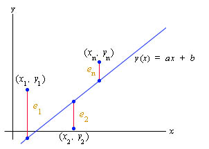
So what are the details behind the applet that you are manipulating above? The least squares best fit of a line to data (also called linear regression) is a means of finding a the best line through a set of data. Consider a set of n data points: (x₁, y₁), (x₂, y₂), ... , (x_n, y_n). We want to select a slope, a, and an intercept, b, that results in a line

that in some sense best fits the data.

The least squares best fit minimizes the square of the error in the distance between the y_i values of the data points and the y value of the line, which depends on the selection of the slope, a, and the intercept, b. We define the error between the data points and the line as:

e_i = y_i - y(x_i) = y_i - (ax_i + b), i = 1,...n.

Let us define the absolute error between each of the data points and the line as

You can see that e_i varies as a and b vary. Below is a graph showing these error measurements.

The least squares best fit is found by finding the minimum value of the function

The technique for finding the exact values of a and b uses Calculus of two variables. The formulae for finding a and b can be found in any book on statistics. A hyperlinked appendix is provided to give you these formulae, but this is only provided for completeness and not as part of this course. You will learn much more about this topic in your Biostatistics course (Biology 215).

Worked Example:

We demonstrate how these errors are computed with the example above for finding the C period in E. coli. The line is given by the formula:

The first datum point is t = 10 and c = 7130. The model predicts c(10) = 6900, so the absolute error between the experimental and the theoretical value is given by

Similarly, we find

We add up the squares of these errors to obtain

You can manipulate the applet and find that this is the smallest value possible.

An additional hyperlinked section is provided to give you some Worked Examples related to the homework problems.

Juvenile Height Revisited

The last lecture section presented data on the average height of a child depending on age. Below is an extension of the applet from the linear section that includes the computation of the square of the error between the linear model and the data for the height of the children. Once again, you can adjust the slope, m, and the intercept, b, in the applet below to find the minimum value of J(m,b), which gives the least squares best fit to the data.

Alternate Image - Alternate link

As noted in the previous section, the resulting least squares best fit to the data is given by the line

and the square of the error is found to be

Calculating Error

There are a number of techniques for computing the error in a measurement. Let X_e be an experimental measurement and X_t be the theoretical value. In this course, most often X_e will be the value from a model that we want to test, while X_t will be results from actual data that we acquire and assume is true. The actual error is simply the difference between the experimental (or model) value and the theoretical (or actual data) value. So the actual error is given by

Often we only need the magnitude of the error or as in the case of the least squares best fit the error is squared making the sign of the error irrelevant. In this case, we use the absolute error, which is simply the absolute value of the difference between the experimental (or model) value and the theoretical (or actual data) value. So the absolute error is given by

More often the error is presented as either the relative error or percent error. This error allows a better comparison of the error between data sets or within a data set with large differences in the numerical values. The relative error is the difference between the experimental (or model) value and the theoretical (or actual data) value divided by the theoretical (or actual data) value, so

The percent error is closely related to the relative error, except that the value is multiplied by 100% to change the fractional value to a percent, so

 References:

[1] J. L. Ingraham, O. Maaloe, and F. C. Neidhardt, Growth of the Bacterial Cell, Sinauer Assoc., Inc., Sunderland, MA, 1983.

[2] Ruth Kavenoff and Brian Bowen, Bluegenes #1, Designergenes Posters, ltd., 1989.

[3] F. C. Neidhardt, Escherichia coli and Salmonella typhimurium: Cellular and Molecular Biology, American Society of Microbiology, Washington, D.C., 1987.