1. Sum of Squares Error
2. Least Squares Best Fit
3. Juvenile Height with Sum of Squares Error

Example 1:

• Two researchers had only a limited set of data, the points (2,2), (5,6), and (8,3).
• Researcher A felt that the model given by

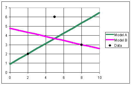
with y increasing with increasing x.

• Researcher B thought that a better model was

with y decreasing with increasing x.

• Sketch the graph of the data points and the two lines.
• Find the sum of squares errors for each of the models.
• Which one is better according to the data?

Solution:

• Recall that for a line y(x) = ax + b, the error is given by e_i = |y_i - y(x_i)| = |y_i - (ax_i + b)|, i = 1, 2, 3.
• The line with the best fit has the smallest sum of the squares of the errors, J(a, b).
• For Model A, J(a, b) is calculated as follows:

J_A = e₁² + e₂² + e₃² = 10.89

• For Model B, J(a, b) is calculated as follows:

J_B = e₁² + e₂² + e₃² = 10.89

• Since J_A = J_B, the two models are equally valid.

Example 2:

• Use the formula in the appendix to find the least squares best fit line for the data in Example 1.
• Which researcher had the right understanding of how y related to x? (Note: These data are clearly insufficient for true research and would require more experimentation as you'll learn in Biostatistics.)

Solution:

The average of the x data values:

The slope a of the best fit line is calculated as follows:

The intercept b of the best fit line can then be calculated.

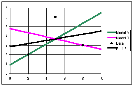
The equation of the best fit line is:

The sum of square errors with this model compared to the data is 8.167, which is lower than the sum of square errors from either Model A or Model B.

Note that since the best fit model shows y increasing with x, Researcher A actually has a more appropriate model than Researcher B. However, more data points are necessary in order to develop a more accurate model of the data.

You can also use Excel to find the best fit line.

Example 3: Often data sets have points that are clearly erroneous due to problems with the experiment (say contamination) or simply a poorly recorded value. If these points are included in the model, then they can result in misleading models.

We saw that growth rates are determined by the slope of a line from our example on juvenile height.

a. Consider the following data set:

The least squares best fit to this data set is given by

Determine the growth rate for this model and find the sum of squares error. Graph the data and the least squares best fit line.

b. Which point is most likely erroneous? When this point is removed, then the new least squares best fit model is given by

Determine the growth rate for this model and find the sum of squares error for this model. What is the percent error (taking the growth rate from the model in Part b. as the actual one) between the computed growth rates?

Solution:

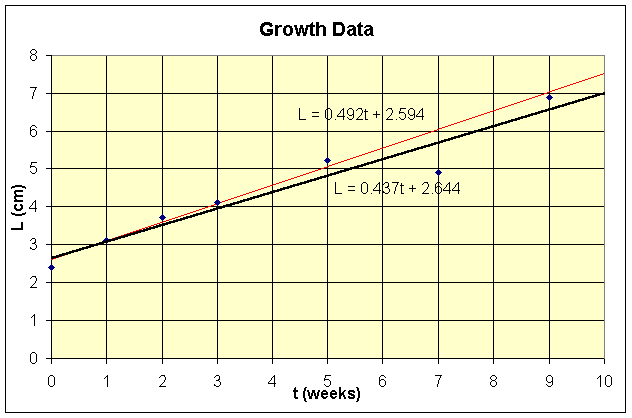
a. The growth rate is represented by the slope of the best fit line, or 0.437 cm/week. The sum of squares error is calculated as follows:

J (a, b) = e₁² + e₂² + e_3² + e₄² + e₅² + e₆² + e₇², where:

So the sum of squares error J =1.0008.

b. From the squares of the errors calculated above, the point with the most error is (7, 4.9), or the second to last point in the data table. Eliminating this point from the data set yields a new best fit line, and a smaller sum of squares error, as shown below.

which is only 9% of the sum of squares error from Part a.

Percent error is calculated as follows:

If the new best fit growth rate is assumed to be the theoretical value, and the old best fit growth rate is the experimental value, the percent error is