![]()
Math 121 - Calculus for Biology I
Spring Semester, 2009
Introduction to the Derivative
San Diego State University -- This page last updated 14-Mar-09
|
|
Math 121 - Calculus for Biology I |
|
|---|---|---|
|
|
San Diego State University -- This page last updated 14-Mar-09 |
|
Introduction to the Derivative
In this section we want to introduce the derivative. There are several ways to view this important concept in Calculus. The previous two sections examined discrete models for population growth. One method, and probably the most common in biological applications, is viewing the derivative as a rate of growth. A second, the more classical approach to the derivative as developed by Newton, is relating the derivative to velocity. A third and more geometric view of the derivative is the tangent line. This section develops the concept of the derivative, and the following sections study techniques for finding the derivative and using it in applications.
The Derivative as a Growth Rate
We begin our study by returning to an example introduced in our section on linear functions. Below is a graph for the heights of girls and boys at the 50th percentile for ages 0 to 18. The original data can be seen at kidsgrowth.com
In the linear section, we noted that the rate of growth is the slope of the line through the data. Over a wide range of ages, this rate of growth is almost constant. However, as the graphs above show, the earliest years show a much higher rate of growth and the later years show a significant slowing in the growth rate. The annual growth rate is easily computed by taking the difference in heights in two successive years, which is the slope of the line connecting the data points. In the early years of life, the data are collected more frequently, every 3 months. If you have quarterly data on height, then you take the difference in the heights between successive measurements and multiply by 4 to obtain the annual growth. In either case, the growth rate g(t) can be approximated by the formula
where t0 is the first age being considered with height at that age being h(t0) and t1 is the second age being considered with its corresponding height of h(t1).
For example, for girls,
|
|
|
|
|
|
|
|
|
|
|
|
Similarly, for small boys,
|
|
|
|
|
|
|
|
|
|
|
|
Below we show the graph of the growth rates for girls and boys from the height graph given above. Notice that initially the growth rate is higher, then it stays almost constant for many years, and finally drops almost to zero. This growth rate being constant is indicative of the heights lying almost on a straight line.
In 1913, Carlson [1] studied a growing culture of yeast.
Below is a table of the population for these yeast (in thousands/cc) measured
at one hour intervals.
|
|
|
|
|
|
|
|
|
|
|
|
|
|
|
|
|
|
|
|
|
|
|
|
|
|
|
|
|
|
|
|
|
|
|
|
|
|
|
|
|
|
|
|
|
|
|
|
|
A graph of these data is presented below.
This graph of the population of yeast shows what is classically called an S-shaped curve. It occurs frequently in biological models (recall the Michaelis-Menten enzyme curve). The population of yeast grows slowly in the beginning, then its growth rate increases to where its a maximum near 8 hours, then decreases and levels off as the population reaches its carrying capacity. Define the population at each hour as P(t).
The growth of the yeast for each hour is computed by taking the difference in the populations at each hour (and dividing by 1 hour). As we did above for the growth of a child, we find the growth of the population by computing
Once again this is the slope of the curve above computed between each of the data points. This can be seen in the graph of the growth function g(t) shown below. If we had more data, then we might expect a smoother growth curve. It is very important to note that the graph of the yeast population (above) and the graph of the growth of the yeast population (below) are different graphs, but are related through the slope of the population graph. The derivative will be the instantaneous growth rate at any time for any population curve.
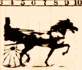
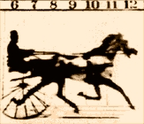
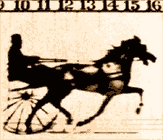
In the 1800s, there was a controversy whether or not a trotting horse ever had all feet off of the ground. This led the photographer Eadweard Muybridge to develop some special photographic techniques for viewing animals and humans in motion by collecting timed sequences of still pictures. When viewed in succession with the same intervening times, these pictures produce an animation of motion, which was a precursor to modern motion pictures. There is a website with several of these classical studies by Eadweard Muybridge. Let us examine the one for a trotting horse.
Our interest here is determining the velocity of the trotting horse. It is often asked how fast a particular animal can run or what speed is a bird flying, but answering this question is much trickier. You should think of how you might determine say the speed of a cheetah hunting a Thompson's gazelle or the velocity of a peregrine falcon diving to catch a pigeon. Below is a blown up sequence from the "trotting horse" movie at the website above. The question is: How fast is the horse trotting?
|
Image 1, time = 0 sec |
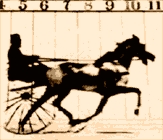
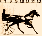
Image 2, time = 0.04sec |
 |
 |
|
Image 3, t = 0.08 sec |
Image 4, t = 0.12 sec |
 |
 |
|
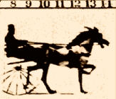
Image 5, t = 0.16 sec |
Image 6, t = 0.2 sec |
 |
 |
|
Image 7, t = 0.24sec |
Image 8, t = 0.28 sec |
 |
 |
|
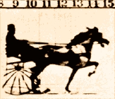
Image 9, t = 0.32 sec |
Image 10, t = 0.36 sec |
 |
 |
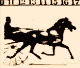
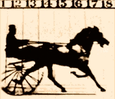
The question above is one about velocity of the trotting horse. Velocity has units of distance divided by time (typically, miles or kilometers per hour or feet or meters per second). Thus, the velocity of the trotting horse is found by computing the distance covered between successive picture frames divided by the time between the pictures. From the frames presented above there is a scale in the background measuring the distance (in feet), and the time between frames is given. If we choose the man's head for a reference point, then we can easily see the position at t0 = 0, satisfies s(t0) = 3.5 ft. At t1 = 0.04, the head is at s(t1) = 4.5 ft. Thus, the velocity is given by
Notice at t2 = 0.08, the head is at s(t2) = 5.6 ft, so the velocity satisfies
which is approximately the same.
An average velocity for the entire sequence of pictures gives the best average velocity for this trotting horse. It is computed by taking the initial and final positions of the head and dividing by the total time between the frames. Thus,
So we see that the velocity is relatively constant over the short time interval of the pictures.
The question would become much more complicated if we asked the velocity of the right front hoof. Clearly, this sequence of pictures is inadequate for properly studying its motion. Does the right front hoof stop or move backwards at any time? How would you answer this question? You would probably want more pictures taken at smaller intervals of time.
Example 4: Falling under the influence of Gravity
The classical study from physics for velocity is the motion of a falling ball. The University of British Columbia website shows a method for producing a series of pictures similar to those for the trotting horse, using a strobe light to capture the motion of a ball.
Rather than choosing the classical approach with a simple ball falling under gravity, let's relate falling under the influence of gravity to the animated cartoon of Wile E. Coyote. We have just viewed Eadweard Muybridge's study of a trotting horse, and an animation of his classical pictures gives a pretty good simulation of motion, yet we saw that even in his pictures there would not be the resolution to answer some of the questions we might ask about the motion of a horse.
In animation, the cartoonist must give the viewer a sense of motion through a series of picture frames also. Obviously, the cartoonist does not have to obey the laws of Physics, yet he must produce a result that allows the viewer to sense motion through a series of snapshots. How many pictures are necessary to give the viewer a reasonable sense of the motion?
In the series below, we actually use the law of gravity to position Wile E. Coyote falling off a cliff that is about 500 feet high. Suppose we choose to look only once every 10 seconds, we see

This does not give us much resolution on the fall of Wile E.Coyote, and makes for little understanding of the velocity of this fall from the cliff. Suppose we examined the fall looking at five second intervals instead.

This is a slight improvement with one additional data point that at 5 seconds he's 400 feet down. (This simulation ignores air resistance on Wile E.) We could at least get an average velocity for part of the fall, but again the resolution and animation is weak. Let us see how the fall looks with one second intervals of time.

This animation gives a better sense of Wile E. Coyote's fall. By superimposing each picture (at the end), we can see that the distance he travelled each second got longer. This resolution allows us to better see the changing velocity as the fall progresses.
The simulation above uses an animation of Wile E. Coyote falling to demonstrate the effect of gravity. The picture frames would be a series of still pictures that put together give us a sense of motion. In this example, we present an applet that simulates a ball falling under gravity (no air resistance) with a strobe light catching the position of the ball at regular time intervals. You can choose the interval of time at which you want to observe the ball by varying the time between the flashes of the strobe light.
Change the time between strobe flashes by entering different values in the window. The left frame shows the position of the ball as it drops, while the right frame graphs the position as a function of time.
source for
dropdistance5f
Alternate link
In the next section, we shall develop the geometric perspective of the derivative as a tangent line. However, the formulae above should be reminding you of the equations we used to find the slope of a line. Thus, our geometric viewpoint of a derivative will be equivalent to what we have discussed above.
Worked Examples are provided to aid in the understanding of this material and help with the homework exercises.
[1] T. Carlson Über Geschwindigkeit und Grösse der Hefevermehrung in Würze. Biochem. Z. 57: 313-334, 1913.