![]()
Math 336 - Mathematical Modeling
Spring Semester, 2000
San Diego State University -- This page last updated 1-Feb-00
|
|
Math 336 - Mathematical Modeling |
|
|---|---|---|
|
|
San Diego State University -- This page last updated 1-Feb-00 |
|
Outline of Chapter
In the first section we showed one of the simplest of mathematical models, which is relating one variable to another using a straight line or linear relationship. Often this is a reasonable approximation to biological data over a limited domain. This section examines the most common technique for fitting a straight line to data known as linear least squares best fit or linear regression. (The term regression comes from a pioneer in the field of applied statistics who gave the least squares line this name because his studies indicated that the stature of sons of tall parents reverts or regresses toward the mean stature of the population.)
Finding the C period for E. coli
|
|
|
The bacterium Escherichia coli is capable of very rapid proliferation.(See the animated gif above to see actual E. coli growing and dividing.) Under ideal growing conditions, these bacteria can divide every 20 minutes. Its genetic material is organized on a large loop of DNA (3,800,000 base pairs) that is replicated in two directions, starting from a site called oriC and terminating about halfway around the loop.(The figure to the right above shows a picture by R. Kavenoff and B. Bowen of the DNA of E. coli.[2]) Bacteria differ from eukaryotic organisms (most commonly studied in your first course in biology) in their replication cycle. Biologists denote the time for the DNA to replicate as the C period and the time for the two loops of DNA to split apart, segregate, and form two new daughter cells as the D period. Since the C period is often 35-50 minutes and the D period is over 25 minutes, you can readily see that the beginning of the C period (called the initiation of DNA replication) must occur several cell cycles in advance for rapidly growing cultures of bacteria. (There can be as many as 8 oriCs in a single E. coli bacterium because of this overlap of activity in the replication process.) See references [1] and [3] below for more information.
Since rapidly growing cultures of E. coli are continually replicating DNA, a pulse label of radioactive thymidine can be used (along with several drugs to halt initiation of replication and cell division) to determine the length of the C period. Below are some data from the laboratory of Professor Judith Zyskind (at San Diego State University) measuring the radioactive emissions, c in counts/min (cpm), from a culture of E. coli that have been treated with drugs at t = 0, then pulse labeled at various times following the treatment.
|
t (min) |
10 |
20 |
30 |
40 |
|
c (cpm) |
7130 |
4580 |
2420 |
810 |
We would like to estimate the C period using a simple linear model,
c = at + b.
(The actual modeling process requires a more complicated mathematical model using integral Calculus.) The t-intercept gives an approximate value to the C period for this culture of E. coli. Adjust the slope, a, and the intercept, b, in the applet below to find the minimum value of J(a,b), which gives the least squares best fit to the data.
The resulting least squares best fit to the data is given by the line
c = -211t + 9010.
The t-intercept is 42.7, so this model estimates the C period as 42.7 min.
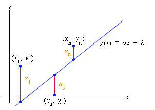
So what are the details behind the applet that you are manipulating above? The least squares best fit of a line to data (also called linear regression) is a means of finding a the best line through a set of data. Consider a set of n data points: (x1, y1), (x2, y2), ... , (xn, yn). We want to select a slope, a, and an intercept, b, that results in a line
y(x) = ax + b,
that in some sense best fits the data.
The least squares best fit minimizes the square of the error in the distance between the yi values of the data points and the y value of the line, which depends on the selection of the slope, a, and the intercept, b. Let us define the error between each of the data points and the line as
ei = |yi - y(xi)| = |yi - (axi + b)|, i = 1,...n.
You can see that ei varies as a and b vary. Below is a graph showing these error measurements.
The least squares best fit is found by finding the minimum value of the function
The technique for finding the exact values of a and b uses Calculus of two variables. The formulae for finding a and b can be found in any book on statistics. A hyperlinked appendix is provided to give you these formulae.
The last section began with a discussion of the DNA replication cycle in E. coli. DNA provides the genetic code for all of the proteins, which are used either directly or indirectly for all aspects of the growth, maintenance, and reproduction of the cell. The synthesis of proteins follows the processes of transcription and translation.
Transcription of a bacterial gene is a controlled sequence of steps, where the protein, RNA polymerase, reads the genetic code and produces a complementary messenger RNA (mRNA) template. This mRNA is a short-lived blueprint for the production of a specific protein that has some particular activity in the bacterial cell.
Translation of the mRNA in bacteria begins shortly after transcription starts, with ribosomes (consisting of ribosomal RNA and ribosomal proteins) reading the triplet codons on the mRNA. The ribosome sequentially assembles a series of amino acids (based on the specific codons read), which form a polypeptide. It is believed that the physical properties of the atoms in the polypeptide cause it to fold passively into a tertiary structure that either becomes an active protein or, when combined with other elements from the cell (such as another polypeptide or lipids), becomes an active protein or enzyme.
![]()
![]()
The rate of growth of a bacterial cell depends on the rate at which it assembles all of the components inside the cell. However, the rate of production of different components inside the cell varies depending on the length of time it takes for a cell to double. The table below shows the doublings/hr, denoted m, and the rate of mRNA synthesis/cell, denoted rm.
|
|
|
|
|
|
|
|
|
|
|
|
|
|
Due to the instability of the mRNA, its rate of production closely approximates the rate of growth of a cell. The data are seen to lie almost on a straight line passing through the origin, which suggests a linear mathematical model of the form
rm = am,
for some value of a, which is the slope of the linear model.
A linear least squares best fit of this model to the data above can be used to find the slope of the model, a. The sum of the squares of the errors is computed using the formula from the previous section. From the data above and the model, we find each of the error terms as follows:
e12 = (4.3 - 0.6a)2, e22 = (9.1 - a)2, e32 = (13 - 1.5a)2,
e42 = (19 - 2a)2, and e52 = (23 - 2.5a)2.
We expand each of these squared terms and add them together. The resulting equation is
J(a) = 13.86a2 - 253.36a + 1160.3,
where J(a) is a quadratic function representing the sum of the squares of the errors. As noted in the previous section, the best fit of the model is found by finding the smallest value of J(a), which is the vertex of this quadratic equation.
Below is an applet, where on the left you can manipulate the slope, a, of the line to fit the data (as before), while on the right you observe the value of the quadratic function, J(a). Notice that the best fit to the data occurs at the vertex of the parabola traced by J(a). The vertex of the parabola above is (a, J(a)) = (9.14, 2.45).
1. A limited set of data is collected and shown in the table below:
| t | 1 | 3 | 5 | 8 |
| y | 4 | 3 | 6 | 5 |
Two researchers interpreted these data differently. Researcher A felt that a good model is given by
y = 0.4x + 2.6,
while Researcher B thought the biological evidence suggests a better model, which satisfies the equation
y = -0.4x + 6.2.
a. Sketch the graph of the data points and the two lines. Which model shows an increasing relationship between the variables and which one shows a decreasing relationship?
b. Find the sum of the squares of the errors for each of the models. Which one is better according to the data?
c. Use the formula in the appendix to find the least squares best fit line for the data in this problem. Which researcher had the right understanding of how y related to x?
2. A research project on the plankton examines the light intensity filtered by the plankton as a function of the depth of the water. The data are shown in the table below:
| depth (m) | 1 | 1.5 | 2 | 3 | 4 | 5 |
| intensity | 0.32 | 0.29 | 0.27 | 0.27 | 0.15 | 0.11 |
a. The least squares best fit to this data set is given by the equation
I = -0.0524 d + 0.3792,
where d is the depth in meters and I is the intensity of light filtered by the plankton. Find the sum of squares error. Graph the data and the least squares best fit line.
b. On observing the graph of the data, one point seemed obviously erroneous. Which point is most likely erroneous? When this point is removed, then the new least squares best fit model is given by
I = -0.0536 d + 0.3728.
Find the sum of squares error for this model. If the model in Part b. is taken to be the actual model, then find the percent error between the slopes of the models in Parts a.\ and b.