|
|
Math 636 - Mathematical Modeling |
|
|---|---|---|
|
|
San Diego State University -- This page last updated 25-Sep-01 |
|
|
|
Math 636 - Mathematical Modeling |
|
|---|---|---|
|
|
San Diego State University -- This page last updated 25-Sep-01 |
|
This section continues the development of some ecological models for two species that are competing for the same resources. As we did in the previous section, an equilibrium analysis is performed. The analysis is extended to provide a geometric understanding of equilibria. Nullclines are introduced, which will allow easier qualitative analysis of 2-Dimensional differential equations. The model is linearized about the equilibria to determine the behavior of the model near the equilibria. The end of this section discusses how the parameters are identified for the two species model of competition, where the exact solution of the differential equations are unknown.
Chemostat with Two Yeast Populations
The last two sections discussed building a mathematical model for cultures of yeast in a chemostat. The study has focused on the work of G. F. Gause [1] in his book Struggle for Existence, where he performed controlled experiments on cultures of the standard brewers yeast, Saccharomyces cerevisiae, and a slower growing yeast, Schizosaccharomyces kephir. The previous section analyzed the mathematical models for the monocultures, which provides information on the growth rates of these species under low (Malthusian growth) and high (intraspecies competition and logistic growth) densities when they are only affected by their own populations and the conditions of the experimental set up. In this section, the models are extended to determine how these species interact when competing for the limited resources, which is called interspecies competition.
Below we repeat the series of tables, graphs, and equations for the two monocultures of S. cerevisiae and S. kephir. The mathematical models are the nonlinear least squares best fit to the data of the Gause experiments (with the data shifted by 6 hours from the original data). The first table and graph combines two experiments of Gause using only S. cerevisiae in the culture.
Table for Single Species Culture of Saccharomyces cerevisiae
|
Time (hr) |
0
|
1.5
|
9
|
10
|
18
|
18
|
23
|
25.5
|
27
|
34
|
38
|
42
|
45.5
|
47
|
|
Volume |
0.37
|
1.63
|
6.2
|
8.87
|
10.66
|
10.97
|
12.5
|
12.6
|
12.9
|
13.27
|
12.77
|
12.87
|
12.9
|
12.7
|
The graph shows the best fitting solution to the data, and its formula is given below.
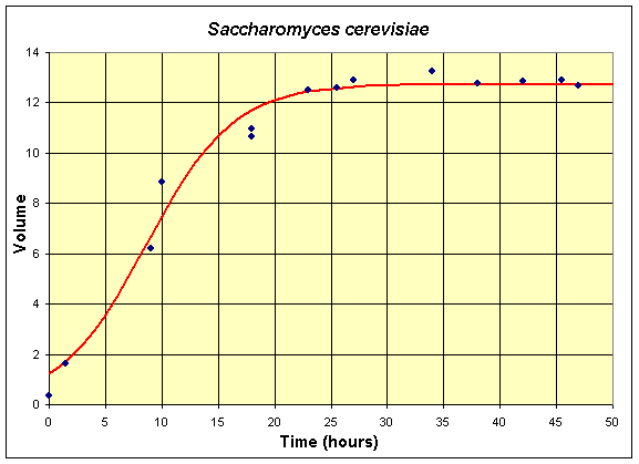
If we let X(t) be the population for S. cerevisiae, then the differential equation for this yeast population that best fits these data is given by

which has the solution (see logistic growth solution section and parameter fit)
![]()
The second table and graph combines two experiments of Gause using only S. kephir in the culture. To match with the data for the experiment with S. cerevisiae, these data are also shifted by 6 hours from the original (which had the first measurement at 15 hours after innoculation). These data are collected over a much longer time period because of the slow growing nature of S. kephir.
Table for Single Species Culture of Schizosaccharomyces kephir
|
Time (hr) |
9
|
10
|
23
|
25.5
|
42
|
45.5
|
66
|
87
|
111
|
135
|
|
Volume |
1.27
|
1.0
|
1.7
|
2.33
|
2.73
|
4.56
|
4.87
|
5.67
|
5.8
|
5.83
|
The graph shows the best fitting solution to the data, and its formula is given below.
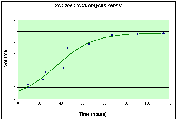
If we let Y(t) be the population for S. kephir, then the differential equation for this yeast population that best fits these data is given by

which has the solution (see logistic growth solution section and parameter fit from the homework)
![]()
Finally, we present a table that shows the competition of S. cerevisiae and the slower growing S. kephir that Gause performed in two experiments. Once again the data are shifted by 6 hours from the original experiment to match the first time when data was actually collected after innoculation of the yeast cultures.
Table for Mixed Species Culture of Saccharomyces cerevisiae and Schizosaccharomyces kephir
|
Time (hr) |
0
|
1.5
|
9
|
10
|
18
|
18
|
23
|
25.5
|
27
|
38
|
42
|
45.5
|
47
|
|
Volume (S. cerevisiae) |
0.375
|
0.92
|
3.08
|
3.99
|
4.69
|
5.78
|
6.15
|
9.91
|
9.47
|
10.57
|
7.27
|
9.88
|
8.3
|
| Volume (S. kephir) |
0.29
|
0.37
|
0.63
|
0.98
|
1.47
|
1.22
|
1.46
|
1.11
|
1.225
|
1.1
|
1.71
|
0.96
|
1.84
|
We need a model that finds the populations of these two species competing for the limiting resources. The single species models provide some information on the parameters in the model, but this mixed population experiment adds complications to the mathematical model, which are developed below. A graph of the data and the best fitting solution to a competition model is shown after the development of the model.
Let us create a mathematical model for two competing species. Let X(t) be one species of yeast and Y(t) be a second species of competing yeast. In the absence of the second species of yeast, we would expect X(t) to satisfy a logistic growth model. Thus, the dynamics for its growth is given by the equation:
The first term, a1X(t), is the standard Malthusian growth, and the second term, -a2X2(t), is the loss due to crowding. It is also known as intraspecies competition. In the Gause experiments listed above, the single species experiments for S. cerevisiae allowed us to find the parameters a1 and a2.
However, we are assuming that there is competition from a second species, interspecies competition. This is modeled very much like the loss term in the predator-prey model. Thus, to the logistic model given above, we need to add the interspecies competition term, -a3X(t)Y(t), so the equation for the dynamics of the first species of yeast is given by
Simlarly, the growth of the second species of yeast satisfies the differential equation
![]()
Again, the Gause experiments for the single species experiments for S. kephir allowed us to find the parameters b1 and b2. It remains to find the parameters for the interspecies competition, a3 and b3.
The two differential equations above create a system that describes the dynamics of two competing species of yeast. So what does this system of differential equations suggest for possible outcomes for these two competing species of yeast? This system of differential equations cannot be solved exactly, so we need to resort to our techniques of qualitative analysis along with some numerical methods to find the remaining parameters.
As we have seen before, the equilibria are found by setting the derivatives equal to zero. Thus, we need to solve the system of nonlinear equations

for the equilibria Xe and Ye. The solution to this system of nonlinear equations is given by
and
Ye = 0 or b2Ye + b3Xe = b1.
Algebraically, if Xe = 0, then either Ye = 0 or Ye = b1/b2. The symmetry of the relations show that when Ye = 0, then there is another equilibrium at Xe = a1/a2. These three equilibria all have extinction of at least one of the species. There is one other equilibrium solution that allows coexistence of both species, which results from solving simultaneously the equations a2Xe + a3Ye = a1 and b2Ye + b3Xe = b1. The result is the fourth (coexistence) equilibrium

provided each of these are positive. There are multiple cases to be considered when either or both of these quantities are negative or zero. A bifurcation (change in behavior of the system of differential equations) occurs when any of these parameters varies and results in one of the quantities above to become zero. Bifurcation studies will be discussed later in this course.
For the Gause experiment with the two yeast species S. cerevisiae and S. kephir, the data seem to indicate a coexistence of the the two species with a leveling off of the populations (though not as clearly as in the single species experiments). Estimates of the value for this coexistence equilibrium provide an initial guess that allows us to perform a least squares best fit to the data using techniques that are developed in the numerical methods section for two differential equations below. The resulting system of differential equations with the best fitting initial conditions is given by

A graph of the data and the solutions to these differential equations is shown below.
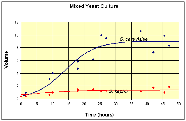
This simulation shows that at t = 50, the model for the population of S. cerevisiae is at X(50) = 8.97 and the model population of S. kephir is at Y(50) = 1.35.
From our discussion above, this system of differential equations has the four equilibria given by
Xe = 0 and Ye = 0
Xe = 0 and Ye = 5.880
Xe = 12.74 and Ye = 0
Xe = 10.37 and Ye = 0.8469
Thus, at t = 50, the simulation of the model has not gone to any of these equilibria, but is closest to the coexistence equilibrium. In fact, the maximum population of S. cerevisiae is reached at t = 44 with X(44) = 8.98, then this population begins declining. By t = 500, the population of S. cerevisiae is X(500) = 0.01, while the population of S. kephir is Y(500) = 5.83. So it follows that over very long periods of time, S. kephir will drive S. cerevisiae to extinction. This process is known as competitve exclusion and is the most frequent outcome of two competing species. Despite the fact that S. kephir grows more slowly, it has an inherent competitve advantage over S. cerevisiae and dominates given sufficient time.
A geometric method for finding the equilibria and extending our understanding of the solutions of the differential equations is to find the nullcines of the differential equations. The definition of a nullcline is simply when the derivative is equal to zero, which is what the equations above show. Graphically, we draw the nullclines in the XY-plane. Below we show a graph for our competition model of yeast with the nullcines and the solution in the phase space.
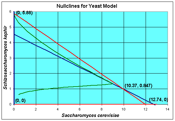
In the solution of the equilibria above, we factored the right hand side of the differential equations, then set them equal to zero. If we graph each of the factors, then we find that dX/dt = 0 produces the blue lines above, while dY/dt = 0 produces the red lines. The solution must crosses the blue lines vertically, since dX/dt = 0. The solution must crosses the red lines horizontally, since dY/dt = 0. Note that these conditions mean that the solutions cannot become negative (as we would expect).
The nullcline analysis can be extended to provide more information about the behavior of the system of differential equations. The regions separated by the nullclines have monotonic behvior. In the diagram above, both X(t) and Y(t) are increasing in the region closest the origin. The solution must continue until it hits either the blue line or the red line above this region (with the exception of one solution that connects the origin with the coexistence equilibrium, which is called the separatrix). If the solution crosses the blue line, then the sign of the derivative of X(t) changes and the solution moves to the left. It can be readily seen that moving in this direction, the solution is unable to cross the red nullcline above it, so the solution is trapped and heads towards the equilibrium at (0, 5.88), which implies that S. kephir will drive S. cerevisiae to extinction. Similarly, if the solution crosses the red line above the region near the origin, then the sign of the derivative of Y(t) changes and the solution moves to the downward. It can be readily seen that moving in this direction, the solution is unable to cross the blue nullcline above it, so the solution is trapped and heads towards the equilibrium at (12.74, 0), which implies that S. cerevisiae will drive S. kephir to extinction.
Clearly, if the solution begins in either of the regions above the region where both X(t) and Y(t) are increasing, then the solution is trapped as discussed above. If the solution begins in the fourth region above the equilibrium, then it can be easily shown that the solution moves monotonically down and to the left until it crosses into one of the regions where it becomes trapped and moves to one of the equilibria, where one of the populations is extinct and the other is at its carrying capacity. Once again, there is one solution that goes directly to the coexistence equilibrium along the separatrix. This behavior is known in ecological circles as competitive exclusion, where only one species is allowed to exist when limited resources are available with the stronger competitor winning out.
Below we show the direction field to help the reader view the behavior of the trajectories of the differential equations.
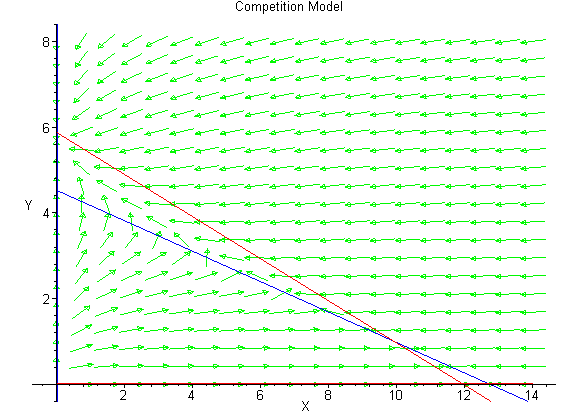
There are a number of good software tools for viewing phase plane solutions of 2-D systems of differential equations. One that can be downloaded from Rice and uses MatLab (possibly Java) is available through this hyperlink.
The next step in our analysis is to linearize the differential equation near each of the equilibria. A Maple worksheet is provided to show how this is done in Maple along with a hyperlink to a copy of the worksheet in HTML. If we define the model for competition by
Numerical Methods for Fitting the Parameters
The model for competition includes terms for interspecies competition, which had the parameters, a3 and b3. We used the monoculture experiments to obtain the growth rates, a1 and b1, and the intraspecies competition parameters, a2 and b2. These were readily found because we know the solution of the logistic growth equation and can use nonlinear solvers to determine the least squares best fit of data to the nonlinear function that solves the logistic growth equation. This was demonstrated in the previous section. However, the competition model has no solution, so what numerical techniques will allow fitting the two species competition experiments to the model above.
We can numerically solve the system of differential equations for the model of competition. However, the parameters must be fixed for the numerical solvers to be computed. Thus, we begin our numerical fitting of the parameters by taking an initial guess to the parameters and numerically solving the system of differential equations. This numerical solution is evaluated at the times where data were collected and the sum of squares error is computed. Next a nonlinear fitting routine searches to select a new set of parameters that lowers the sum of squares error. The process is repeated until a minimum is reached within some tolerance. This gives the least squares best fit to the data. Below we show how to perform these calculations using an Excel spreadsheet and a MatLab program.
Excel Fitting the Parameters
For the purposes of this example, we decided to chose a relatively simple method for numerically solving the system of differential equations for the mixed populations of yeast, the Improved Euler's method. Since this fitting of the parameters is highly nonlinear, we must begin with a reasonable guess at the initial parameters. (More details appear in a link to an Excel spreadsheet on the numerical fitting of the parameters. These are referred to below.)
The unknown parameters in this model are the initial populations X(0) and Y(0) and the interspecies competition parameters, a3 and b3. The initial choice for the initial populations X(0) and Y(0) are the ones given by the experiments, X(0) = 0.375 and Y(0) = 0.29. To find the interspecies competition parameters is more complicated. In this experiment, we observe that the populations in the mixed culture appear to level to some coexistence equilibrium (which we saw does not occur over a long period of time). It is fortunate that for this experiment we have a fast growing species that eventually dies out, which allows the experiment to approach a quasi-equilibrium near the coexistence equilibrium. We approximate the coexistence equilibrium by averaging the last 6 data points in the experiment. This yields a quasi-equilibrium
Xe = 9.25 and Ye = 1.31
Since we are assuming that we know the parameters a1, a2, b1, and b2, then the formulae above for finding the coexistence equilibrium produces two nonlinear equations with the two unknowns a3 and b3. The solution of these two nonlinear equations (using Maple) gives the initial estimates for the parameters
a3 = 0.054 and b3 = 0.0048.
The initial conditions appear in cells G6 and I6 in the Excel spreadsheet provided, while the parameters a3 and b3 appear in the cells G5 and I5.
As noted above, the next step is the numerical solution of the system of differential equations. The Improved Euler's method is used for this calculation because of its simplicity. The Improved Euler's method uses a fixed stepsize and satisfies the following algorithm:

where the y is a vector of the approximate solutions for X and Y and f is a vector function given by the right hand side of the differential equations above, including the unknown parameters that are minimized. In order to not require too many steps, a relative large stepsize h = 0.5. On the Excel spreadsheet, the Improved Euler's method is implemented in the cells B16 through G16 and down.
The next step is the computation of the sum of square errors. The data points are given at each time ti for S. cerevisiae , Xd(ti), and for the S. kephir, Yd(ti). The sum of square error is computed by the formula

On the Excel spreadsheet, the sum of square error appears in cell L34. This cell is the one that we apply the Excel solver routine to minimize subject to changing the cells for the parameters (G5, G6, I5, and I6).
The result of this complex minimization problem produces the parameters
X(0) = 0.4184 and Y(0) = 0.6315
a3 = 0.05711 and b3 = 0.004803.
The sum of squares error produced by these parameters, which is minimized by Excel's solver, and is equal to 19.40482. Note that this error includes errors produced by using the Improved Euler's method, so even changing the stepsize would vary this result.
MatLab Fitting the Parameters
One major problem with the solution produced by Excel is the weakness in the numerical solution to the system of differential equations using the Improved Euler's method, especially with a large stepsize of h = 0.5. MatLab has several built in ordinary differential equation solvers. For the purposes of this section, we take advantage of its ode23 solver.
The MatLab approach begins very much as we did for Excel with reasonable initial guesses for the parameters. We have to enter the data, where there was a minor hitch as the ode23 solver could not handle two different data points with the same times, hence we sorted the data, leaving the one repeated data point at the end. this would be handled by the match.m file that we created. Below we list the m-files that created.
The first file gives the vector function for the right hand side of the differential equations, including the parameters which can be varied.
function dydt = compet(t,y,a1,a2,a3,b1,b2,b3)
% Competition Model for Two Species
tmp1 = a1*y(1) - a2*y(1)^2 - a3*y(1)*y(2);
tmp2 = b1*y(2) - b2*y(2)^2 - b3*y(1)*y(2);
dydt = [tmp1; tmp2];
Next we write the match file to sort data and the sum of squares error function.
function M = match(data1,data2)
% If you have a data set with repeated data (which fails
in ode23),
% then this program find indices of repeated times.
n1 = length(data1);
n2 = length(data2);
M = [];
for i = (n1+1): n2
for j = 1:n1
if data1(j) = = data2(i)
M = [M j];
end
end
end
function J = leastcomp(p,tdatam,tdata,xdata,ydata)
global A1 A2 B1 B2
n1 = length(tdatam);
n2 = length(tdata);
[t,y] = ode23(@compet,tdatam,[p(1),p(2)],[],A1,A2,p(3),B1,B2,p(4));
errx = y(:,1)-xdata(1:n1)';
erry = y(:,2)-ydata(1:n1)';
J = errx'*errx + erry'*erry;
M = match(tdatam,tdata);
m1 = length(M);
for i = 1:m1
J = J + (y(M(i),1)-xdata(n1+i))^2 + (y(M(i),2)-ydata(n1+i))^2;
end
We enter the vectors for the data and the initial parameter values, beginning with a statement to make the variables A1, A2, B1, B2 global.
global A1 A2 B1 B2
td = [0 1.5 9 10 18 23 25.5 27 38 42 45.5 47 18]
tds = [0 1.5 9 10 18 23 25.5 27 38 42 45.5 47]
xd = [0.375 0.92 3.08 3.99 4.69 6.15 9.91 9.47 10.57 7.27 9.88 8.3 5.78]
yd = [0.29 0.37 0.63 0.98 1.47 1.46 1.11 1.225 1.1 1.71 0.96 1.84 1.22]
A1 = 0.2586 A2 = 0.0203 B1 = 0.0574 B2 = 0.0098
p = [0.375 0.29 0.054 0.0048]
Finally we use the fminsearch routine as follows:
[p,fval,exitflag] = fminsearch(@leastcomp,p,[],tds,td,xd,yd)
The result converged to a best set of parameters
X(0) = 0.4110 and Y(0) = 0.6258
a3 = 0.05697 and b3 = 0.004758.
The sum of squares error produced by these parameters, which is minimized by Excel's solver, and is equal to 19.311. This sum of square errors is smaller than the one from Excel, but then a very diffferent differential equation solver with much higher accuracy was used, so a different set of parameters and sum of square error (not necessarily lower) are expected. Note that this change in the parameters would shift the position of the coexistence equilibrium to
Xe = 10.26 and Ye = 0.8848
This creates a minor shift in all of the numbers computed above, but no change in the qualitative behavior. All of the graphs would look the same as the differences are only a few percent.
[1] G. F. Gause, Struggle for Existence, Hafner, New York, 1934.
[2] G. F. Gause (1932), Experimental studies on the struggle for existence. I. Mixed populations of two species of yeast, J. Exp. Biol. 9, p. 389.