Direction Field and Linear Analysis for Competition Model
We begin by creating the direction field and the nullclines for the webpage. We begin by entering the differential equations and creating the direction field.
> dex := diff(x(t),t) = 0.2586*x(t) - 0.0203*x(t)^2 - 0.05711*x(t)*y(t);
![]()
> dey := diff(y(t),t) = 0.05744*y(t) - 0.009768*y(t)^2 - 0.004803*x(t)*y(t);
![]()
>
with(DEtools):
with(plots):
Warning, the name changecoords has been redefined
>
P1 := dfieldplot([dex,dey],[x(t),y(t)], t=0..20, x=0..14, y=0..8, arrows=MEDIUM, title=`Competition Model`,
color=GREEN):
Create the nullclines. Then show all graphs together.
>
eq1 := 0.2586 - 0.0203*X - 0.05711*Y;
eq2 := 0.05744 - 0.009768*Y - 0.004803*X;
![]()
![]()
> Y1 := solve(eq1=0,Y); Y2 := solve(eq2=0,Y);
![]()
![]()
> P2 := plot({Y1,1E12*(X-0.05)}, X = 0..14, Y = 0..8, color = BLUE):
> P3 := plot({0.01,Y2}, X = 0..14, Y = 0..8, color = RED):
> display({P1,P2,P3});
![[Maple Plot]](images/nulletc7.gif)
Next we find the equilibria. We simply note that (0, 0) is one of them. The others are found as follows:
> xelog := solve(subs(Y=0,eq1=0),X);
![]()
This gives the S. cerevisiae carrying capacity.
> yelog := solve(subs(X=0,eq2=0),Y);
![]()
This gives the S. kephir carrying capacity.
> te := solve({eq1=0,eq2=0},{X,Y});
![]()
> coexx := rhs(te[2]); coexy := rhs(te[1]);
![]()
![]()
Above is the coexistence equilibrium.
Next we define the right hand sides of the differential equations.
> f1 := (X,Y) -> 0.2586*X - 0.0203*X^2 - 0.05711*X*Y;
![]()
> f2 := (X,Y) -> 0.05744*Y - 0.009768*Y^2 - 0.004803*X*Y;
![]()
As an example, we perform a Taylor series expansion about each of these functions around the carrying capacity equilibrium for S.cerevisiae . This shows the local linearization.
> taylor(f1(X,0),X=xelog);
![]()
> taylor(f1(xelog,Y),Y=0);
![]()
> taylor(f2(X,0),X=xelog);
![]()
> taylor(f2(xelog,Y),Y=0);
![]()
We want to compare the above computation with the one derived by computing the Jacobian matrix and evaluating at the equilibria. In addition, we find the eigenvalues and eigenvectors at all 4 equilibria.
> with(linalg):
Warning, the name adjoint has been redefined
Warning, the protected names norm and trace have been redefined and unprotected
> A := vector([f1(X,Y),f2(X,Y)]);
![]()
> J := jacobian(A, [X,Y]);
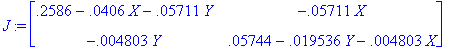
> X := 0: Y := 0: J0 := J(0,0);
![J0 := matrix([[.2586, -0.], [-0., .5744e-1]])](images/nulletc21.gif)
> eigenvects(J0);
![]()
This gives an unstable node .
> X := xelog: Y := 0: J1 := J(xelog,0);
![J1 := matrix([[-.2586000002, -.7275195076], [-0., -...](images/nulletc23.gif)
> eigenvects(J1);
![]()
This gives an stable node.
> X := 0: Y := yelog: J2 := J(0,yelog);
![J2 := matrix([[-.772311220e-1, -0.], [-.2824368550e...](images/nulletc25.gif)
> eigenvects(J2);
![]()
This gives another stable node .
> X := coexx: Y := coexy: J3 := J(coexx,coexy);
![J3 := matrix([[-.2014788273, -.5668204841], [-.4803...](images/nulletc27.gif)
> eigenvects(J3);
![]()
This gives a saddle node .