|
|
Math 122 - Calculus for Biology II |
|
|---|---|---|
|
|
San Diego State University -- This page last updated 23-Mar-04 |
|
|
|
Math 122 - Calculus for Biology II |
|
|---|---|---|
|
|
San Diego State University -- This page last updated 23-Mar-04 |
|
The solutions of differential equations involve finding the inverse of some problem stated with derivatives. Many of these inverse problems cannot be solved, but there are special forms of differential equations where integration provides the solution. The last section showed that differential equations with only time varying functions are easily integrated to find the solution. In this section, we examine a class of differential equations that can be separated into two integration problems to form the solution of the differential equation.
Malthusian Growth Model
The Malthusian growth model has a simple exponential form for a solution. However, a simple Malthusian growth model with a single growth rate does not predict human populations very well. In the section for discrete Malthusian growth models, we showed that by adding a time varying component to the model to account for changes in growth rates due to changing societal conditions, the mathematical model predicts the population much more accurately and indicates some of the changes affecting future population growth.
Let us compare two differential equation models of population growth that are based on the U.S. census data from our earlier section. The basic Malthusian growth model with a constant growth rate is the simplest model and has the form
which has a solution of the form
For the U. S. census data, if we want to best match the data in 1790 and 1990 (where the population is 3.9 million in 1790 and 248.7 million in 1990), then the best fit to this Malthusian growth model is P0 = 3.9 (million), t0 = 1790, and r = 0.020776. This gives the solution
If we modify this model to allow the growth rate to vary linearly with time, then the model becomes
where k(t) = at + b is a linear function.Though this is still a linear differential equation, it cannot be solved using the techniques developed in the earlier section.
How do we solve this type of differential equation? Also, what are the best constants a and b that fit the data for the U. S. population in 1790 and 1990?
Separable Differential Equations
We noted earlier that differential equations are difficult in general to solve. At this point, we can only solve a couple types of differential equations. These include linear differential equations (e.g., Malthusian growth model, radioactive decay, and simple Newton's law of cooling) and differential equations with only time varying functions (e.g., falling objects). The next easiest type of differential equation to solve is called a separable differential equation.
Consider the differential equation
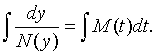
If the function f(t,y) has the special separable form with f(t,y) = M(t)N(y), then we can implicitly solve the differential equation by integration. If we think of y ' as the quotient of differentials dy/dt, then we can separate the differential equation in the following manner:
Notice that the left hand side has only the dependent variable y, while the right hand side has only the independent variable t.
The solution is obtained by integrating both sides. Thus, the solution is given by
Example 1: Consider the differential equation

Solution: Separate the variables t and y, so that only t and dt are on the right hand side and only y and dy are on the left hand side. The resulting integral form is
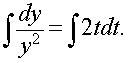
We solve these two integrals using our integration techniques to give
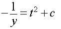
Note that you only need to put one arbitrary constant, despite solving two integrals. This is easily rearranged to give the solution in explicit form
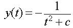
Note that it may not be possible to find the explicit answer y(t), but when possible it is better to give the answer in this easier form.
There are more examples worked in the Worked Examples section.
Modified Malthusian Growth Model
If we let k(t) = at + b in the model for the growth of the U. S. population with time varying growth rate, then we can write the modified Malthusian growth model as follows:
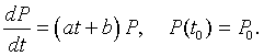
This equation is clearly separable, so the solution is obtained in the following manner;
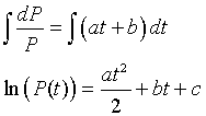
for some constant c. By exponentiating the solution above, we obtain
There are only two data values, which are given from the census data in 1790 and 1990. However, the integrated expression has 3 parameters to fit (a, b, and c). With the initial condition, P(t0) = P0, we can show that the solution is given by
(Note that the b in this expression is not the same as the b in the previous expression.) We would like to fit this model to the U. S. census data with the population in 1790 as 3.9 million and in 1990 as 248.7 million. From the data in 1790, we can use the second form of the solution with P0 = 3.9 (million) and t0 = 1790 to give
This still leaves the two parameters a and b to find, but only one remaining data value given. Thus, this problem needs additional information to solve.
The best parameter values are found by taking the logarithms of the U.S. census data and fitting a quadratic through the data. (The U. S. census data can be found in the discrete dynamical systems section in the Math 121 lecture notes. The quadratic fit to the logarithm of the population is seen by the formula formed by integrating the separated differential equation above.) The best parameters for the U. S. census data are a/2 = -6.992x10⁻⁵ and b = 0.03476.
We would like to compare the Malthusian growth model from above given by
![]()
and the nonautonomous Malthusian growth model given by

The table below shows the populations (in millions) predicted by each of these models at the dates 1790, 1900, 1990, and 2000.
|
Model |
1790 |
1900 |
1990 |
2000 |
|
U.S.
Census Data |
3.9 |
76.0 |
248.7 |
281.4 |
|
Malthusian |
3.9 |
38.3 |
248.7 |
306.1 |
|
Nonautonomous |
3.9 |
77.2 |
248.7 |
266.3 |
From the table, it can be seen that the models were selected to match the U.S. census data at the dates 1790 and 1990. The predictions for 2000, show that the Malthusian growth model is too high by 8.8%, while the nonautonomous Malthusian growth model is too low by 6.1%. (This last decade experienced higher growth than the trend for the previous 5 decades.) Each of the models fails to predict the actual census in 2000 very well. However, for 1900, show that the Malthusian growth model is too low by 49.6%, while the nonautonomous Malthusian growth model is too high by 0.8%. Thus, the Malthusian growth model does a very poor job of predicting the population, while the nonautonomous Malthusian growth model predicts the population quite well. Below we show a plot of the U. S. census data, the simple Malthusian growth model, and the nonautonomous Malthusian growth model.
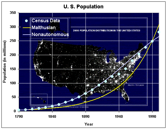
From the graph it is clear that the modified Malthusian growth model is much better at simulating the U. S. census data, so provides a better tool for predicting future population. Notice that the value of b is close to the value for the Malthusian growth rate of the U. S. population near 1790.
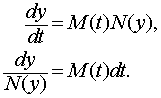
Most cells are primarily water. The loss of water due to dessication is primarily through the surface of the cell. We saw in the laboratory comparing length of a dog to the surface area and weight that surface area varies proportionally to length squared, while volume varies according to length cubed. Thus, the rate of change of the volume is proportional to the surface area to the 2/3 power. This suggests that an appropriate model for the dessication of a cell would be given by the following differential equation:
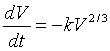
where V is the volume of the water in the cell, t is time, and k is an appropriate constant.
Suppose that we are given that the initial volume of water in the cell is V(0) = 8 mm3. Suppose that 6 hours later the volume of water has decreased to only 1 mm3. Solve this differential equation, finding k and determining when all of the water has left the cell.
Solution: This is a nonlinear separable differential equation, so we separate the variables as follows:
Upon integration, we obtain
which can be written
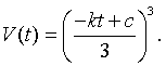
The initial condition gives
The condition at t = 6 gives
Thus, the solution to this problem is
It becomes clear that the solution vanishes (all the water evaporates) at t = 12. Below is a graph of the solution.