1. Introduction
2. Blood Pressure
3. Model for Arterial Pressure
4. Radioactive Decay
5. Worked Examples
6. Newton's Law of Cooling
7. Pollution in a Lake

Introduction

This section examines several examples of linear first order differential equations that we are able to solve. The applications are to Arterial pressure, Radioactive decay, Newton's Law of cooling, and Pollution in a lake.

Blood Pressure

When you have your blood pressure measured, you are given two numbers. A reading of 120/80 is considered normal for humans. So how are those numbers generated and what can we infer from them? The numbers for blood pressure reflect the force on arterial walls and are given in units of mm of Hg, which is how high a column of mercury rises. This pressure is clearly generated by the beating of the heart.

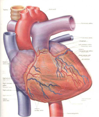
We begin discussion of the cardiac cycle with the pulmonary circulation. Blood flows from the body into the right atrium and into the right ventricle before going through the pulmonary artery to the lungs to be oxygenated. After the blood exchanges O₂ and CO₂ in the lungs, it returns through the pulmonary vein to the left atrium. The pressure in the pulmonary vein and the left atrium at this point is between 5 and 15 mm of Hg, which is very low compared to the pressures described above as arterial pressure.

Blood flows into the left ventricle until it is almost full. The heart is fairly rigid even when relaxed, so the pressure within the ventricle increases only slightly during the filling process. The right atrium contracts, then the AV valve between the atrium and the venricle closes. At this point, the heart receives an electrical signal, which causes ventricular contraction, beginning the process called systole. As the walls of the left ventricle contract, the pressure in the ventricle increases until it "blows" open the aortic valve and blood rapidly flows into the aorta under this high pressure (systolic pressure). As pressure rises in the aorta, the AV valve reopens, while the aortic valve closes.

At this point, there is high pressure in the aorta, which forces the blood into the other arteries of the body. As the blood flows through the body, the aortic pressure drops to its low pressure, the diastolic pressure. At this lowest pressure, the cycle begins anew with the rapid rise to the systolic pressure and the drop over the next second (at rest) to the diastolic pressure. The blood pressure drops as the blood branches from the aorta to the brachial arteries to the smaller arteries, like the arterioles, to the capillaries, then returning to the heart via the veins at a relatively low pressure. The flow through the capillaries is fairly constant with a relatively constant pressure maintained.

Your blood pressure is actually measured in one of the brachial arteries in your arm, which is very representative of the pressure in the aorta. (However, the blood pressure readings can vary depending on which arm is used, and if major differences occur, then it is suggestive of certain disease states.) We will model the arterial pressure, P_a(t), during a single beat of the heart and try to determine the important modeling parameters in the system.

Model for Arterial Pressure

Our model begins with the blood ejected from the left ventricle into the aorta. The cardiac output, Q, represents the average amount of blood pumped by the heart (in liters/min). The stroke volume, V, is the amount of blood pumped by the heart during one beat (liters/beat). In the model, this is the amount that enters the aorta at the beginning of systole. If T is the duration of a heart beat, then we can relate flow from the cardiac output to the stroke volume by the relationship

Note that 1/T is the heart rate in beats/min. When the left ventricle completes pumping the blood into the aorta and the aortic valve closes, then we are at the maximum pressure of the blood in the aorta, which is reflected in the major brachial arteries. We denote this maximum pressure, P_sys.

The blood pressure begins to fall as the blood flows through the arteries. The rate of flowing of the blood depends on the resistance of a blood vessel. The resistance is comprised of three major components: 1. Viscosity of the blood, 2. Length of the vessels, 3. Radius of the blood vessels. The viscosity of the blood is relatively constant, except under diseased states like erythrocytemia (or when athletes take erythropoietin or EPO to overstimulate the production of red blood cells). Similarly, the length of the blood vessels are relatively constant, except for when conditions like pregnancy or amputation occur. Thus, the main factor that changes resistance of the blood flow is change in the radius. Blood pressure therefore becomes a valuable tool for detecting narrowing of the blood vessels by hypertension or atherosclerosis.

Experimentally, it has been observed that systemic blood flow, Q_s, is proportional to the difference between the arterial and venous pressures (P_a(t) - P_v(t)) with the proportionality dependent on the resistance. If R_s is the systemic resistance (mm Hg/liter/min), then we have the following equation:

 

To simplify the model, we take advantage of the fact that venous pressures are very low, so we approximate the systemic flow by the equation:

Compliance is the stretchability of a vessel, which is a property that allows a vessel to change the volume it can hold in response to pressure changes. The higher the compliance the easier it is for a vessel to expand in response to increased pressure. Thus, resistance and compliance have a roughly inverse relationship. Experimentally, the arterial volume, V_a, is roughly equal to the compliance, C_a, times the arterial pressure. Thus,

We are now ready to create a differential equation that describes the arterial pressure. The flow representing the change in the arterial volume is given by the difference between the rate of flow entering the aorta and the rate of flow from the aorta. However, since the aortic valve is closed during systole, no blood is entering the aorta. Thus, we have the following differential equation:

or

But from above, we have V_a (t) = C_a P_a(t), so

Thus, these equations can be put together to give a differential equation describing the arterial pressure:

This differential equation is similar to the Malthusian growth model that we examined in the previous section. The solution to this initial value problem is given by:

This solution is valid for times t between 0 and T.

For this model to be valuable for diagnostic purposes, we need to be able to find the physiological parameters for compliance, C_a , and resistance, R_s. The physiological quantities that can be measured directly are:

1. The heart rate or pulse, 1/T,

2. Cardiac output, Q, using a cardiac output recorder or doppler sonogram,

3. The systolic and diastolic pressures, P_sys and P_dia.

The compliance is from the stroke volume, V, which satisfies:

But V = QT, so it follows that the compliance is computed from the known physiological parameters by the formula:

We know that the diastolic pressure occurs just before the next heart beat. From the model it follows that

This equation can be solved for the resistance, R_s, giving

For a normal person, we have the a pulse of approximately 70 beats/min (1/T), a cardiac output of Q = 5.6 (liters/min), and systolic and diastolic pressures of P_sys = 120 mm Hg and P_dia = 80 mm Hg, respectively. Thus, it is easy to compute the compliance and resistance for a normal person as

Variations in these parameters from the normal values can be used for determining certain medical conditions and be helpful for suggesting various treatments.

Radioactive Decay

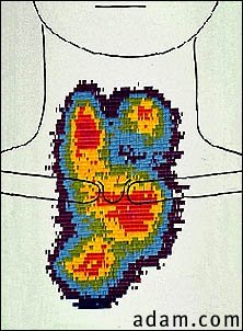
Radioactive elements play an important role in many biological applications. Many experiments use radioactive tracers to determine what sequence of molecular events occurred. For example, ³H (tritium) can be used to tag certain DNA base pairs, which can then be added to mutant strains of E. coli that are unable to manufacture one particular DNA base. By treating the culture with the appropriate antibiotics, one can use the radioactive signal to determine how much DNA was replicated under a particular set of experimental conditions. Radioactive iodine is often used to detect or treat thyroid problems in humans and animals. In most cases, the experiments are run in such a way that radioactive decay is not an issue. (³H has a half-life of 12.5 yrs or ¹³¹I has a half-life of 8 days.)

One important application of radioactive decay is the dating of biological specimens. While an organism is living, it is continually changing its carbon with the environment. (Plants directly absorb CO₂ from the atmosphere, while animals get their carbon either directly or indirectly from plants.) Gamma radiation that bombards the Earth keeps the ratio of ¹⁴C to ¹²C fairly constant in the atmospheric CO₂. The ¹⁴C that entered a living organism can be used to determine how much time has passed since it has died. It has been determined that radioactive carbon, ¹⁴C, decays with a half-life of 5730 years, i.e., in 5730 years the quantity of ¹⁴C decreases to half its original amount. Living tissue shows a radioactivity of about 15.3 disintegrations per minute (dpm) per gram of carbon, which means that 5730 years after the organism has died, it will exhibit only half or 7.65 dpm per gram of carbon. (eg. Shroud of Turin)

Let R(t) represent the number of dpm per gram of carbon from an ancient object. The loss of ¹⁴C from a sample at any time t is proportional to the amount of ¹⁴C remaining. Thus, the amount of ¹⁴C is directly related to R(t) which satisfies the differential equation

From our solution for the Malthusian growth model, it is clear that this differential equation has the solution, R(t) = 15.3e^-kt, where k = ln(2)/5730 = 0.000121.

Example: Suppose that an object is found to have a radioactive count of 5.2 dpm per g of carbon. Find the age of this object.

From the solution above

Thus, t = ln(2.94)/k = 8915 yr, so the object is about 9000 yrs old.

More examples of Malthusian growth, radioactive decay, Newton's law of cooling, and pollution in a lake are found in the hyperlinked Worked Examples section.

Newton's Law of Cooling

After a murder (or death by other causes), one of the first things that the forensic scientist does is to take the temperature of the body. A little later the temperature of the body is taken again to give the investigator an idea of the rate at which the body is cooling. These two (or more) data points can be used to extrapolate back to when the murder occurred. The property that is being applied is known as Newton's Law of Cooling. Newton's Law of Cooling states that the rate of change in temperature of a cooling body is proportional to the difference between the temperature of the body and the surrounding environmental temperature. Thus, if T(t) is the temperature of the body, then it satisfies the differential equation

The parameter k is dependent on the specific properties of the particular object (body in this case), T_e is the environmental temperature, and T₀ is the initial temperature of the object.

Example: Let us suppose that a murder victim is found at 8:30 am and that the temperature of the body at that time is 30^oC. Assume that the room in which the murder victim lay was a constant 22^oC. Suppose that an hour later the temperature of the body is 28^oC. Use this information to determine the approximate time that the murder occurred.

We know that the normal temperature of a human body when it is alive is 37^oC. From the model for Newton's Law of Cooling and the information that is given, if we set t = 0 to be 8:30 am, then we need to solve the initial value problem

Suppose that we make a change of variables. Let z(t) = T(t) - 22, then z'(t) = T '(t), so the differential equation above becomes

But this is just the radioactive decay problem that we just solved. Thus, the solution is given by

However, z(t) = T(t) - 22, so T(t) = z(t) + 22 or T(t) = 22 + 8 e^-kt.

We use the second piece of information to determine the constant k. T(1) = 28 = 22 + 8 e^-k, so 6 = 8 e^-k or e^k = 4/3. Thus, k = ln(4/3) = 0.2877.

It only remains to find out when the murder occurred. At the time of death, the body was 37^oC. So we need to solve

for t. Equivalently, 8 e^-kt = 37- 22 = 15 or e^-kt = 15/8 = 1.875. This gives

From this information, we can conclude that the murder occurred about 2 hours and 11 minutes before the body was found, which places the time of death at around 6:19 am.

Pollution in a Lake

One of the most urgent problems in modern society is how we reduce the pollution and toxicity of our water sources. These are very complex issues that require a multidisciplinary approach and are often politically very intractable because of the key role that water plays in human society and the many competing interests. In this section we will examine only a very simplistic model for pollution of a lake, but it should demonstrate some basic elements from which more complicated models could be built and analyzed.

Consider the scenario of a new pesticide that is applied to fields upstream from a clean lake with volume V. We assume that a river receives a constant amount of this new pesticide into its water, and that it flows into the lake at a constant rate, f. This assumption implies that the river has a constant concentration of the new pesticide, p. Assume that the lake is well-mixed and maintains a constant volume by having a river exiting the lake with the same flow rate, f, that the inflowing river has. We will use this information to set up and solve a linear first order differential equation for the concentration of the pesticide in the lake, c(t).

The key to studying pollution problems of this type is setting up a differential equation that describes the mass balance of the pollutant. Descriptively, per unit time we examine

The amount entering is simply the concentration of the pollutant in the river times the flow rate of the river. To see this we look at the units associated the concentration of the pollutant, p, which are stated in mass/volume. (For example, we might have something like mg/m³. The flow rate, f, has units of volume/time. (For example, we might have m³/day.) Thus, fp gives us the amount entering the lake per unit time, which by assumption is simply a constant.

The amount leaving has the same flow rate, f. Since the lake is assumed to be well-mixed, the concentration in the outflowing river will be equal to the concentration of the pollutant in the lake, c(t). The product f c(t) gives the amount of pollutant leaving the lake per unit time. Thus, if a(t) is the amount of pollutant in the lake at any time t, then a differential equation describing a(t) is given by:

However, we would like this differential equation to be simply described by the concentration of the pollutant in the lake. Since we are assuming that the lake maintains a constant volume V, we have the relationship that c(t) = a(t)/V, which also implies that c'(t) = a'(t)/V. Dividing the above differential equation by the volume V, we have

Since we are assuming that the lake is initially clean, then the initial condition for this differential equation is given by c(0) = 0.

One solves this differential equation in exactly the same manner as solving the problem we saw before for Newton's Law of cooling. Notice that the constant f/V acts like the constant k in Newton's law of cooling, while p acts like the constant T_e. The equation above can be rewritten in the form of Newton's Law of cooling:

Now we make the substitution, z(t) = c(t) - p in a manner similar to before. The derivatives z'(t) = c'(t). The initial condition becomes z(0) = c(0) - p = - p, the initial value problem in z(t) becomes,

The solution to this problem is again like the solution to the radioactive decay problem and can be seen as

Since z(t) = c(t) - p, the solution is easily solved to produce

The exponential decay of the second term in this solution shows that as t becomes "large," the solution approaches p. This is exactly what you would expect, as the entering river has a concentration of p.

Example: Let us work the above problem with some specific conditions. Suppose that you begin with a 10,000 m³ clean lake. If the river entering has a flow of 100 m³/day and the concentration of some pesticide in the river is measured to have a concentration of 5 ppm (parts per million), then we can form the differential equation describing the concentration of pollutant in the lake at any time t and solve it. Find out how long it takes for this lake to have a concentration of 2 ppm.

In a second part of the example, let us suppose that when the concentration reaches 4 ppm, the pesticide is banned. For simplicity, assume that the concentration of pesticide drops immediately to zero in the river. (We are also assuming that the pesticide is not degraded or lost by any means other than dilution.) Find how long until the concentration reaches 1 ppm.

Solution: The differential equation for this problem is given by

We let z(t) = c(t) - 5, then the differential equation becomes,

This has a solution

To find how long it takes for the concentration to reach 2 ppm, we solve the equation

This is equivalent to

Solving this for t, we obtain

For the second part of the problem, there is no pollutant in the river and the initial concentration in the lake is assumed to be 4 ppm. The new initial value problem becomes

In this case, we don't need a substitution as the differential equation above is already in the form of a radioactive decay problem. This has the solution

To find how long it takes for the concentration to return to 1 ppm, we solve the equation

Solving this for t, we obtain

The above discussion for pollution in a lake fails to account for many significant complications. There are considerations of degradation of the pesticide, stratefication in the lake, and uptake and reentering of the pesticide through interaction with the organisms living in the lake. The river will vary in its flow rate, and the leeching of the pesticide into river is highly dependent on rainfall, ground water movement, and rate of pesticide application. Obviously, there are many other complications that would increase the difficulty of analyzing this model. In the next section we will examine how to handle certain complications in this model.