1. Growth of Bacteria
2. Logistic Growth Model
3. Solution of Logistic Growth
4. Qualitative Behavior of Differential Equations 
5. Worked Examples
6. Left Snails
7. References

This section examines nonlinear differential equations using qualitative analysis techniques. Finding analytical solutions to differential equations can be very difficult or impossible, yet often the behavior of the equations can be examined from a qualitative perspective to determine types of behavior, which can lead to insight into modeling problems. In the Math 121 notes, we found that studying equilibria of discrete dynamical systems allowed us to understand much about the behavior of those models. Similarly, qualitative analysis of differential equations can provide valuable insight to complicated biological models.

We begin with the classic example of the logistic growth model, using data from an experiment on bacteria. Equilibria for the model are found and analyzed. A discussion of these techniques is given.

Growth of Bacteria

Bacteria grown in a laboratory are innoculated into a broth, then grown for a period of time. Typically, the growth pattern of any bacterial culture follows a regular pattern. The culture has a lag period as the innoculated culture adjusts to the new growing conditions. This is followed by a period of exponential growth, where the bacterial population satisfies the Malthusian growth model. As the population of bacteria increases, certain nutrients become limiting (or there is a build up of waste products that limit growth). The bacterial cell growth slows, and the culture enters a phase called stationary growth. This is characterized by the population leveling off with the culture using different pathways to survive the lean times.

In the previous semester, we studied the discrete logistic growth model that showed this type of behavior under certain conditions on the parameters. However, the discrete logistic growth model could only be simulated and not solved explicitly. Growth of bacteria is a much more continuous process, so their growth is better characterized by a differential equation. In this section, we will develop the continuous logistic growth model for growth of bacteria and show several techniques for analyzing the model and relating it to experimental data.

Professor Anca Segall in the Department of Biology at San Diego State University has done many experiments on the bacterium Staphylococcus aureus, a fairly common pathogen that can cause food poisoning. Standard growth cultures of this bacterium satisfy the classical logistic growth pattern discussed above. Below we present the data from one experiment in her laboratory (by Carl Gunderson), where a normal strain is grown using control conditions and the optical density (OD₆₅₀) is measured to determine an estimate of the number of bacteria in the culture.

t (hours)	0	0.5	1	1.5	2	2.5	3	3.5	4	4.5	5
OD650	0.032	0.039	0.069	0.110	0.170	0.229	0.261	0.288	0.309	0.327	0.347

Below is a graph of the data (showing a stained culture of Staphylococcus aureus) and the logistic growth model that fits the data. It is clear that the model reasonably well matches the actual biological data.

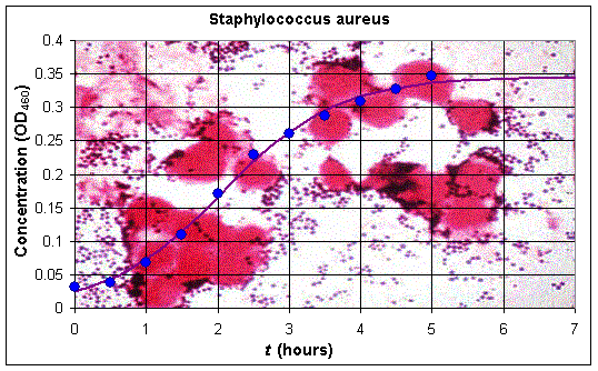
(The picture is from Kenneth Todar at the University of Wisconsin.)

Logistic Growth Model

In this experiment, we see that the population of the bacteria begins by growing quite rapidly, but then levels off. Thus, a model for the population growth should have a component corresponding to Malthusian growth and a term accounting for the crowding effects when the nutrient supply has diminished. Recall that the continuous Malthusian growth model was given by the simple differential equation

In our earlier studies, we saw that the discrete logistic growth model was given by

The term rP_n corresponds to the Malthusian growth, while the term -rP_n²/M is a quadratic term accounting for the crowding effects. As in the arguments made for going from the discrete Malthusian growth model to the continuous Malthusian growth model, where the time interval between n and n+1 becomes small, the continuous logistic growth model follows from the equation above and can be written 

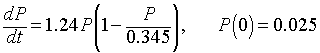
This differential equation was first introduced by the Belgian biologist Verhulst [2], so it is sometimes referred to as the Verhulst equation. A nonlinear least squares fit to Anca Segall's data in the graph above gives the specific logistic growth model

(Finding the parameters for this system uses a nonlinear least squares routine. To learn more about fitting the parameters to the logistic growth model, lecture notes are available from my website.)

Can we solve this differential equation?

There is a solution to the logistic growth differential equation, which can be found in a hyperlink to this section (Solution to the Logistic Growth Model). In fact, there are a couple of methods that can solve this differential equation, either separation of variables (which then uses special integration techniques) or Bernoulli's method. However, since many differential equations cannot be solved or involve complicated methods, we want to develop simpler techniques to understand the qualitative behavior of differential equations.

Qualitative Behavior of Differential Equations

The continuous logistic growth model can be analyzed without finding the exact solution. The techniques follow a similar analysis to the discrete dynamical systems. We first examine the differential equation to find the equilibria, then we determine the behavior of the solutions near those equilibria. Below we detail a typical analysis using the logistic growth equation.

Consider the logistic growth equation:

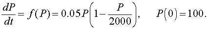
We begin by drawing a graph of the function on the right hand side of the differential equation, f(P).

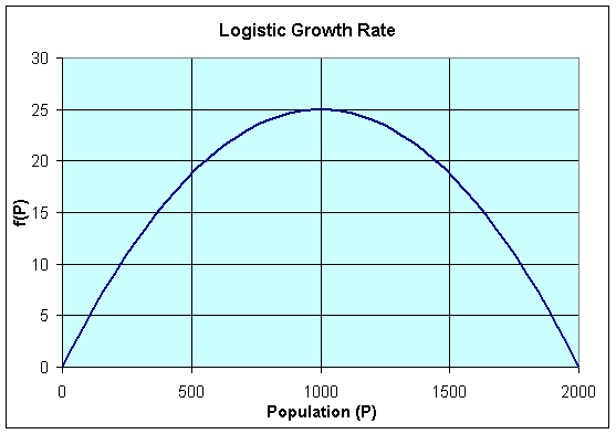
The graph of f(P) shows a parabola that intersects the P-axis at P = 0 and P = 2000. These P-intercepts are where f(P) = 0 or

This means that there is no change in the growth of the population or the population is at equilibrium. This is the first step in any qualitative analysis of a differential equation. Find all equilibria for the differential equation, which are simply all points where the derivative of the unknown function is zero.

The graph of f(P) gives us more information about the behavior of the logistic growth model. As noted above, the equilibria occur at P_e = 0 and P_e = 2000. Notice that to the left of P_e = 0, f(P) < 0, while to the right of P_e = 0, f(P) > 0. Thus, when P < 0, dP/dt < 0 and P is decreasing. (Note that this region is outside the region of biological significance.) When 0 < P < 2000, then dP/dt > 0 and P is increasing. Furthermore, we can see that the greatest increase in the growth of the population occurs at P = 1000, where the vertex of the parabola occurs.When P > 2000, then again dP/dt < 0 and P is decreasing.

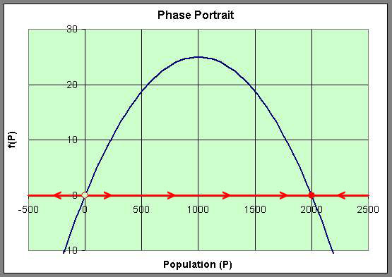
This information allows us to draw what is called a Phase Portrait of the behavior of this differential equation along the P-axis. The behavior of the differential equation is denoted by arrows along the P-axis, which are easily directed by whether the function f(P) is positive or negative. We use a solid dot to represent an equilibrium, which solutions of the differential equation approach asymptotically, and an open dot represents an equilibrium, where solutions nearby move away from the equilibrium. This is diagrammed below using the graph of f(P).

We can easily sketch the behavior of the solutions as functions of time using this phase portrait. Below is a graph of the solutions P(t) with t being the independent variable. The equilibria give rise to horizontal lines (meaning that P(t) does not change with time). When the initial values of P have the phase portrait pointing to the left, then the solution is decreasing, while arrows to the right on the phase portrait have the solutions increasing. The solutions are not allowed to cross paths in the time-varying diagram shown below.

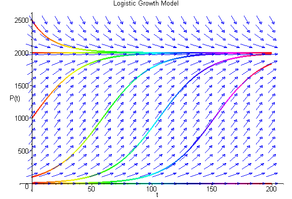
 The solutions above show that all positive initial conditions result in solutions eventually tending towards the equilibirum at 2000. The slope of the solution at any time can be seen in the figure above with the slope matching the value of f(P).

There are more Worked Examples through the usual hyperlink.

Left Snails

Stephen Jay Gould wrote many articles for Natural History on various issues of evolution and was a leading voice against the teaching of "Creation Science." He was also an expert on the evolution of gastropods. The shell of a snail exhibits chirality, which means that the snail shell develops either a left-handed (sinistral) or right-handed (dextral) coil relative to the central axis. In [3], he writes that the Indian conch shell, Turbinella pyrum, is primarily a right-handed gastropod. However, left-handed shells exist and are "exceedingly rare." (The Indians view the shells as right-handed from their perspective, which makes the rare shells very holy.) The Hindu god "Vishnu, in the form of his most celebrated avatar, Krishna, blows this sacred conch shell to call the army of Arjuna into battle." So why does nature favor snails with one particular handedness? Gould notes that the vast majority of snails grow the dextral form.

One mathematical model discussed in the book by Clifford Henry Taubes [4] gives a simple mathematical model to predict the bias of either the dextral or sinistral forms for a given species.

• Assume that the probability of a dextral snail breeding with a sinistral snail is proportional to the product of the number of dextral snails times sinistral snails.
• Assume that two sinistral snails always produce a sinistral snail and two dextral snails produce a dextral snail. Assume that a dextral-sinistral pair produce dextral and sinistral offspring with equal probability.

One could and should debate these assumptions. Note that the first assumption implicitly assumes that given a choice of mates a dextral snail is twice as likely to choose a dextral snail than a sinistral snail. (You can check this implication using basic probability.) It would be useful to have real experimental verification of these assumptions.

Let p(t) be the probability that a snail is dextral. Taubes presents the following model that qualitatively exhibits the behavior described by the assumptions above.

where a is some positive constant. We would like to see the behavior of this differential equation and determine what its solutions predict about the chirality of populations of snails.

Though the differential equation above could be solved using separation of varibles and some integration techniques, the solution is not particularly easy to obtain. However, by using the geometric approach afforded by our qualitative analysis techniques, this differential equation can be analyzed relatively easily to determine why snails are likely to be in either the dextral or sinistral forms.

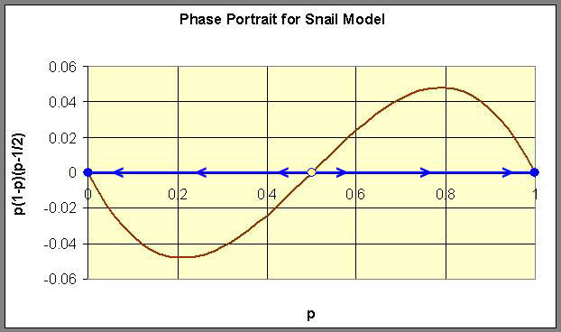
The analysis begins by graphing the function of p on the right hand side of the differential equation. From the graph below, we see that the p-intercepts are 0, 1/2, and 1. Thus, the equilibria for this model are p_e = 0, 1/2, and 1. In addition, we see that the function is negative for 0 < p < 1/2 and positive for 1/2 < p < 1. It follows that all solutions of the differential equation decrease whenever 0 < p < 1/2 and increase whenever 1/2 < p < 1. Thus, we have that the equilibrium at p_e = 1/2 is unstable (denoted by the open circle), and the equilibria at p_e = 0 and 1 are stable (denoted by the closed circles). The phase portrait of this model is shown on the p-axis with the graph of the function on the right hand side of the differential equation drawn to indicate the direction the arrows should be pointing.

Below we show the actual solutions as drawn by Maple for a collection of different initial conditions using the solution space with t as the independent variable and p as the dependent variable. These solutions are shown below.

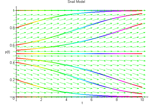
From both of the diagrams above it is easy to see that for this model, the solutions tend toward one of the stable equilibria, p_e = 0 or 1. In the case that the solution tends toward p_e = 0, then the probability of a dextral snail being found drops to zero, so the population of snails all have the sinistral form. When the solution tends toward the equilibrium p_e = 1, then the population of snails virtually all have the dextral form. This is what is observed in nature suggesting that our model exhibits the behavior of the evolution of snails. This does not mean that the model is a good model! It just means that the model exhibits the basic behavior observed experimentally from the biological experiments.

References

[1] T. Carlson Über Geschwindigkeit und Grösse der Hefevermehrung in Würze. Biochem. Z. 57: 313-334, 1913.

[2] P. F. Verhulst, "Notice sur la loi que la population suit dans son accroissement," Corr. Math. et Phys. 10 (1838), 113-120.

[3] S. J. Gould, "Left Snails and Right Minds," Natural History, April 1995, 10-18, and in the compilation "Dinosaur in a Haystack" ( 1996)

[4] C. H. Taubes, Modeling Differential Equations in Biology, Prentice Hall, 2001.