1. Basic Examples
2. Bifurcation
3. Allee Effect

This section uses the qualitative analysis techniques for studying differential equations. A couple of basic examples are shown to illustrate the methods of finding equilibria, determining their stability, and drawing a phase portrait. Next these techniques are applied to a model of populations that exhibit the Allee effect, such as the thick-billed parrot or guacamaya, Rhynchopsitta pachyrhycha, of the Sierra Madre Occidental in Mexico.

Basic Examples

Example 1: Consider the differential equation given by

Find all equilibria and determine the stability of those equilibria. Sketch the phase portrait and show typical solutions in the x and t solution space.

Solution: We begin by finding the equilibria for this differential equation. The equilibria are found by setting the right hand side of the differential equation equal to zero. Thus, we must solve

which happens when the argument of the sine function is np, so px = np or

 where n is an integer. Thus, there are equilibria at every integer value of x. Below is the phase portrait of this differential equation, showing the graph of the right hand side of the differential equation to indicate the direction of the arrows for the phase portrait. It shows that each of the even integers produce an unstable equilibrium and the odd integers give stable equilibria.

 

The graph below shows typical solutions for several initial conditions.

 

Example 2: (Bifurcation) This example illustrates an important idea in qualitative analysis known as a bifurcation of behavior of the differential equation. Bifurcations are when some parameter in the differential equation changes the qualitative behavior. (In this case, we show what is called a supercritical pitchfork bifurcation.) The differential equation has a different number of equilibria dependent on the parameter a in the equation. We consider the differential equation given by the following

where a can be positive, negative, or zero. Find all equilibria and determine the stability of those equilibria for the different possible values of a. For a = +1, sketch the phase portraits and show typical solutions in the x and t solution space.

Solution:

The equilibria are found by setting the right hand side of the differential equation equal to zero. Thus, we must solve

or

There is always an equilbrium at x = 0.

If a < 0, then x = 0 is the only equilibrium. If a > 0, then there are three equilibria given by

The graphs below with a = +1 show that when x = 0 is the only equilibrium, then it is stable. When there are three equilibria, then x = 0 is an unstable equilibrium, while the equilibria, , are both stable. Thus, as the parameter a changes from negative to positive, the differential equation's qualitative behavior changes from having a single stable equilibrium at x = 0 to a differential equation with three equilibria with x = 0 becoming unstable and the other two being stable.

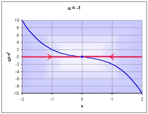
Below we examine the cases a = +1. They are very representative of types of qualititive behavior that can be observed with the differential equation in this example.

Beginning with the case a = -1, we see that the graph is always decreasing and only intersects the x-axis at x = 0. Since the function is positive to the left of zero, this says that the solutions of the differential equation are always increasing toward the equilibrium at x = 0 (though more slowly as the solution approaches zero). On the other hand, the function is negative to the right of zero, so the solutions of the differential equation are always decreasing toward the equilibrium at x = 0 for positive x. The graph below shows the graph of the function and the phase portrait for the differential equation

Typical solutions are shown in the xt-plane below for various initial conditions.

When a = 1, the graph of the right hand side of the differential equation

intersects the x-axis at x = -1, 0, and 1. The function is positive to the left of x = -1, goes negative for -1 < x < 0, then becomes positve again for 0 < x < 1, and ends negative for all x > 1. This information is shown in the phase portrait below with the arrows pointing the direction of the flow of the solution. The result being stable equilibria at x = -1 and 1, and an unstable equilibrium at x = 0 .

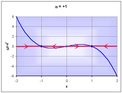
Typical solutions are shown in the xt-plane below for various initial conditions.

The Allee Effect

Example 3: The thick-billed parrot (Rhynchopsitta pachyrhycha) known locally by people of the Sierra Madre Occidental in Mexico as guacamaya or guaca is a gregarious montane bird that feeds largely on conifer seeds, using its large beak to break open pine cones for the seeds. These birds used to fly in huge flocks in the mountainous regions of Mexico and Southwestern U. S. Largely because of habitat loss, these birds have lost much of their original range and have dropped to only about 1500 breeding pairs in a few large colonies in the mountains of Mexico. The pressures to log their habitat puts this population at extreme risk for extinction.

The populations of these birds appear to exhibit a property known in ecology as the Allee effect. These parrots congregate in large social groups for almost all of their activities. The large group allows the birds many more eyes to watch out for predators. When the population drops below a certain number, then these birds become easy targets for predators, primarily hawks, which adversely affects their ability to sustain a breeding colony.

Suppose that a population study on thick-billed parrots in a particular region finds that the population, N(t), of the parrots satisfies the differential equation:

where r = 0.04, a = 10^-8, and b = 2200. Find the equilibria for this differential equation. Determine the stability of the equilibria and draw a phase portrait for the behavior of this model. Describe what happens to various starting populations of the parrots as predicted by this model.

Solution:

The analysis begins by finding the equilibria for this model. The equilibria are found by setting the right side of the differential equation equal to zero or

Since this is in factored form, then this is zero when either of the factors is zero, so either

N_e = 0 or r - a(N_e - b)² = 0.

The first gives the usual trivial solution (N_e = 0), which from the modeling perspective says that when there is no population present, then there is no population in the future (extinction).

The second case can be rewritten

a(N_e - b)² = r or (N_e - b)² = r/a.

By taking the square root of both sides, we have

or

This gives two more equilibria (unless b² = r/a).

We are given that r = 0.04, a = 10^-8, and b = 2200, so the above expression for the two non-zero equilibria becomes

or

N_e = 200 or N_e = 4200.

It follows that our model for thick-billed parrots in a particular region gives the three equilibria

N_e = 0 , 200, and 4200.

Below is a graph of the right hand side of the differential equation (with a blown up insert to show the graph between 0 and 200) that shows the equilibria and their stability. The arrows along the axis indicate the flow of the solution, producing the phase portrait for this model.

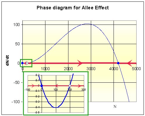
From the phase portrait, we see that the equilibria at 4200 and 0 are stable, while the equilibrium at 200 is unstable. According to this model, if the population is above 200, then it will eventually go to the carrying capacity of this region and reach the stable population of 4200. However, if the population falls below 200, then this model predicts extinction, since the phase portrait shows the solution going to the equilibrium at 0. This agrees with the description for these social birds, which require a critical number of birds to avoid predation. Below this critical number, the predation increases above reproduction, and the population of parrots goes to extinction. (In the diagram above, the solutions with values of N less than zero are meaningless here, but are included mathematically to complete the phase portrait.) Note that if the parrot population is larger than 4200, then this model predicts that their numbers will be reduced by starvation (and predation) until they reach the carrying capacity at the 4200 population level.

This model does not include the effects of humans on the population. Logging the region would decrease the carrying capacity of the population. With fewer trees, there are fewer nesting sites (r decreases) and sources of food (increasing a and decreasing b), so the dynamics of this population would be altered and a different model would be required.