1. Chemostat with Two Yeast Populations
2. Malthusian Growth Model
   1. Solution of the Continuous Malthusian Growth Model
   2. Fitting the Continuous Malthusian Growth Model
3. Logistic Growth Model
4. Qualitative Analysis of the Logistic Growth Model
5. References

One of the easiest introductions to differential equations is through the understanding of population growth models. In the introduction we saw the solution to the Malthusian growth model. In general, populations are limited by various factors. This section examines a couple of models for yeast growth and introduces the ideas of qualitative analysis of differential equations that will follow in the text. The first population study is an experiment of yeast competing for a limited source of nutrient. This section starts with a description of the Gause yeast experiments. Based on the experiments, several mathematical models are discusssed with the techniques required to study them. The models are fit to the data, then a discussion of the qualitative behavior of the models is presented.

Chemostat with Two Yeast Populations

One method for maintaining a culture of yeast used in brewing beer is to create a chemostat. A chemostat is a large vat, where nutrients are pumped into the vat with a constant flow rate, then the growing culture is removed at the same flow rate. Under ideal conditions, a monoculture of yeast grows exponentially at first, then as the population becomes sufficiently large, the concentration of yeast levels off. At a certain level, known as the carrying capacity, the population of yeast balances the supply of nutrient entering the vat. At this stage, the the population (or concentration) of yeast remains constant with as many yeast being born in each unit of time as are flushed out from the chemostat per unit time. These conditions guarantee a constant supply of uniform concentration of the yeast flowing from the chemostat. This allows the brewmaster a consistent supply of the yeast culture, which ensures a uniform product with the desired characteristics. Unfortunately, it is almost impossible to keep a consistent monoculture of the yeast. The vat often gets infected with a competing yeast or bacteria that destroys the uniformity and lowers the quality of the beer. Below is a cartoon illustrating the idea of a yeast culture growing in a chemostat.

Ideally, we would like to develop a mathematical model for the chemostat described above, especially when a contaminating species invades the culture. We begin with an analysis of some classical studies from the 1930s that carefully examine cultures of yeast that have a fixed supply of nutrient. In the book Struggle for Existence, G. F. Gause [1] describes his experiments, which do not use an actual chemostat, but rather changed the nutrient in a closed vessel regularly (every 3 hours). This is roughly equivalent to a chemostat. He performed a number of experiments to test competition of microbial species. One set of experiments examined the standard brewers yeast, Saccharomyces cerevisiae, and a slower growing yeast, Schizosaccharomyces kephir. He tested these organisms in monocultures to find their growth parameters with his experimental set up, then he mixed the cultures to determine how the organisms reacted when they competed in the same nutrient medium. He notes that though he used a standard medium, he was not certain of all the concentrations of the different components in the medium, which complicates the ecological model since the species could be utilizing different components of the medium.

The experiments present an interesting study in population dynamics. For now, we will concentrate only on the two experiments of Gause using only S. cerevisiae in the culture. (Later we may return to Gause's experiments to show competition between two species.) These data are shifted by 6 hours from the original experiment because no data were collected until 6 hours from innoculation of the yeast culture. The innoculation is said to be a single drop from a culture that had been growing for 72 hours and assumed to be at carrying capacity. Notice that Gause measured the volume of the yeast rather than the population, which is probably a better measure of the organism's ability to absorb the nutrients. The volume quoted in the papers only indicated units marked on a centrifuge tube after spinning the culture down, so absolute units are not available.

Time (hr)	0	1.5	9	10	18	18	23	25.5	27	34	38	42	45.5	47
Volume	0.37	1.63	6.2	8.87	10.66	10.97	12.5	12.6	12.9	13.27	12.77	12.87	12.9	12.7

We are now presented with a collection of raw data and would like to explain these data with a mathematical model for the growth of yeast.

How do we create a mathematical model from these data?

We should probably begin this study by finding and analyzing the simplest of population models.

Brewer's yeast, S. cerevisiae, is a simple eukaryotic organism (cells with nuclei) that reproduces asexually by a process of budding. Given an unlimited supply of nutrients (which is the case for lower densities of the yeast), then during any fixed period of time, there is a certain probability that any particular yeast will produce a new bud that will eventually grow to become a mature yeast. There is also a certain probability that a grown yeast will die. From the data on the time, a natural unit of time might be 1/2 hour (though one could argue for minutes or hours equally well). Under conditions where the yeast populations are low relative to the supply of nutrients, then the rate of budding and death should be fairly constant.

Let b be the budding rate per unit volume of yeast (recall that our yeast data above are in volume of cells measured in a centrifuge tube) per unit time. This budding rate will again be in volume units of yeast. Let d be the death rate per unit volume of yeast per unit time. Then the total rate of increase in volume of yeast per unit time per unit volume of yeast (or decrease should the death rate exceed the rate of budding) is given by

Let P(t) be the volume of yeast at time t, then from our discussion above, when the population of the yeast is low relative to the concentration of nutrients, it follows that on average

Biologically, this equation says that the change (difference) in the volume of the yeast over a small period of time is found by taking the rate of growth times the volume of the yeast times the interval of time Dt. The equation above can be rearranged to give

The right hand side of the equation readily transforms into a derivative as we take the limit of Dt tending toward zero. Thus, in the limit this model reduces to the differential equation

This is the continuous Malthusian growth model This model is named after the work of Thomas Malthus (1766-1834). The Malthusian growth model states that the growth of the population is simply proportional to the current population, which is what is written in the equation above.

Solution to the Malthusian Growth Model

The differential equation describing the continuous Malthusian growth model says that the derivative of an unknown Population function P(t) is equal to a constant times the unknown Population function. (The rate of change of a population is proportional to the population.) The only function that we know that is a derivative of itself is the exponential function. We try a solution of the form

where c is an arbitrary constant. But P '(t) is cre^rt, which is rP(t), so satisfies the differential equation. If we add an initial condition P(0) = P₀, then the unique solution becomes

This is another reason why Malthusian growth is often called exponential growth. This solution is equivalent to the solution of the discrete Malthusian growth model with the exception that the time is in units of hours, which corresponding affects the growth rate ^r.

Fitting the Continuous Malthusian Growth Model

The model above is very general, but we would like to match the actual data for the yeast to see how well the continuous Malthusian growth model applies.

Algebraic fit to the data

We use the first and third data points for S. cerevisiae, (t, P) = (0, 0.37) and (t, P) = (9, 6.2) to fit the continuous Malthusian growth model and find the parameters P₀ and r. From the model, the first data point gives

The third data point gives

It follows that

so the continuous Malthusian growth model satisfies

Exponential fit (Linear least squares best fit to logarithm of data)

If we take the first 4 data points from the data on S. cerevisiae, then fit the best straight line through the logarithm of the data. The best straight line fit to the logarithm of the volume data is given by

It follows that

Thus, the best continuous Malthusian growth model is given by

Nonlinear least squares best fit

Finally, if we minimize the sum of the square error between the data and the continuous Malthusian growth model. For the first 4 data points on S. cerevisiae, the least squares functional is given by

where

The solution to this minimization problem gives the parameters

Thus, the best Malthusian growth model for this nonlinear least squares fit is given by

These solutions are completely equivalent to the discrete cases above. Another Excel worksheet is provided by a hyperlink to see the computations. A graph of these models with the data is shown below.

Clearly, these models fit only a small part of the data (the first 4 points were used in the fit), and their behavior is not a very good representation. This is clearly an inadequate mathematical model to describe the dynamics of these experiments.

How do we improve on the Malthusian Growth model to fit these data?

For the most part, yeast are continually growing organisms, which implies that using differential equation models are the most appropriate. For an individual species with a population at time t given by P(t), we can write a general model using a differential equation of the form

for a general function f(t, P), representing the growth rate of the population. (Of course, this is the way that we can write any first order differential equation.) The Malthusian growth model has the form

This equation is classified as a linear constant coefficient differential equation, which given the initial condition P(0) = P₀, has the unique solution

The general differential equation above does not have a solution, so we need to determine what simplifications make sense for the experiments described above.

The Gause yeast experiments are closed systems with a careful design that ideally allows reproducibility. The experimental design with a continuous flow of nutrients and constant environmental conditions indicates the growth rate (reflected in the function f(t, P)) should only depend on the population variable P and not the time t. This implies that our growth model should be an autonomous differential equation of the form

Note that the Malthusian growth model is autonomous and linear.

Consider a Maclaurin series expansion of the function f(P). If we write the first few terms of the series expansion, then

where O(P³) means order of P³. Since the system is closed, when the population is zero, then the population stays at zero (no growth), so

The linear term comes from the Malthusian growth, so

From the data, we know that the population growth rate declines for larger population. In biology, this is known as intraspecies competition. Mathematically, this implies that the next most significant term in the Maclaurin series expansion after the linear growth term must be negative. For reasons that will soon become apparent, we define

If the higher order terms can be ignored, then we have the differential equation given by

This is the logistic growth model.

The development above uses basic mathematical principles, but one can readily argue a similar term from an ecological perspective. In an environment with limited resources, then interactions between individuals results in fighting for those resources. The interaction between two individuals is modeled by the random contact, which is proportional to the product of their density (P²). This interaction is detrimental (or negative) because of the limited resources, so is given by a term of the form -rP²/M, which is the same as listed above from the Maclaurin series approach.

The logistic growth model is a nonlinear differential equation. Most nonlinear differential equations cannot be solved, so we introduce you to the techniques of qualitative analysis of differential equations. However, since the logistic growth equation is solvable, we will also show how to solve this particular equation.

The first step in any qualitative analysis of a differential equation is to find all equilibria (if they exist). Equilibria are found by setting the right hand side of the differential equation equal to zero. Thus,

This means that there is no change in the growth of the population or the population is at equilibrium. In closed population models, one equilibrium is always the zero or trivial equilibrium. If we consider the logistic growth model, then the equilibria, P_e, satisfy

It is easily seen that

The value M is the carrying capacity of the logistic growth model. The Gause experiments do provide good data for the carrying capacity of the yeast. An estimate of the carrying capacity is readily found by averaging the data points after growth of the yeast has leveled off. We can see that the growth has leveled off after about 24 hours, so if we average these data points, we obtain

Thus, the carrying capacity is about 12.9, which matches well with the value of 13.0 reported by Gause.

Phase Portrait

The computations from the previous section on Malthusian growth of S. cerevisiae in the Gause experiments gave an estimated initial volume and growth rate of about

P₀ = 0.7 and r = 0.25,

while the computation above gave the carrying capacity of

M = 12.9.

Since r/M = 0.0194, an reasonable approximation for the logistic growth model is given by the following initial value problem

P ' = f(P) = 0.25P - 0.0194P², with P(0) = 0.7.

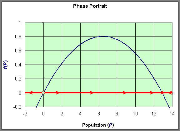
The graph of f(P) gives more information about the behavior of the logistic growth model. As noted above, the equilibria occur at P_e = 0 and P_e = 12.9. Notice that to the left of P_e = 0, f(P) < 0, while to the right of P_e = 0, f(P) > 0. (The slope of the tangent line at P_e = 0 is the eigenvalue, r.) Thus, when P < 0, dP/dt < 0 and P is decreasing. (Note that this region is outside the region of biological significance.) When 0 < P < 12.9, then dP/dt > 0 and P is increasing. Furthermore, we can see that the greatest increase in the growth of the population occurs at P = 6.45, where the vertex of the parabola occurs.When P > 12.9, then again dP/dt < 0 and P is decreasing. (The slope of the tangent line at P_e = 12.9 is the eigenvalue, - r.)

This information allows us to draw what is called a Phase Portrait of the behavior of this differential equation along the P-axis. The behavior of the differential equation is denoted by arrows along the P-axis, which are easily directed by whether the function f(P) is positive or negative. This is diagrammed below using the graph of f(P). The open circle on the P-axis represents the unstable equilibrium, while the full circle on the P-axis represents the stable equilibrium.

We can easily sketch the behavior of the solutions as functions of time using this phase portrait.

Direction Fields

We can easily sketch the behavior of the solutions as functions of time using this phase portrait. Below is a graph of the solutions P(t) with t being the independent variable. The equilibria give rise to horizontal lines (meaning that P(t) does not change with time). When the initial values of P have the phase portrait pointing to the left, then the solution is decreasing, while arrows to the right on the phase portrait have the solutions increasing. The solutions are not allowed to cross paths in the time-varying diagram shown below (uniqueness of the solutions of the differential equation, which we will discuss later).

The solutions above show that all positive initial conditions result in solutions eventually tending towards the equilibirum at 12.9. Note that the third curve from the bottom solves the initial value problem listed above. The slope of the solution at any time can be seen in the figure above with the slope matching the value of f(P). The Maple commands to generate the figure above are given by

> with(DEtools):

> de := diff(P(t),t) = 0.25*P(t) - 0.0194*P(t)^2;

> DEplot(de, P(t), t=0..30, [[P(0)=0], [P(0)=0.2], [P(0)=0.7], [P(0)=2], [P(0)=6], [P(0)=10], [P(0)=16], [P(0)=12.9]],stepsize=.2, title=`Logistic Growth Model`,color=[.3*y(t)*(x(t)-1),x(t)*(1-y(t)),.1], linecolor=t/2,arrows=MEDIUM,color=blue,method=rkf45);

These experiments illustrate a problem when the experimentation does not use the feedback (shown in the introduction to the lectures). The experiments are meant to verify the logistic growth model, yet they were not redesigned after testing against the mathematical model. These experiments lack the very important initial values, which we will see are very important, and there are a paucity of data through the primary growth phase of the yeast. This leads to large margins of error in the choice of some of the parameters.

There is a special hyperlink to a section showing the solution of the logistic growth model. The section below examines how we find the growth parameters for these experiments.

Fitting the Logistic Growth Model - Yeast 

The best technique to fit the experimental data uses a nonlinear least squares method. This section will show how we can fit the data using either an Excel spreadsheet with Solver or MatLab's fminsearch routine.

A nonlinear least squares methods need some reasonable initial estimate before they are likely to converge. From our nonlinear least squares analysis of the Malthusian growth model and the estimate above of the carrying capacity, we obtain a reasonable initial guess using

The solution to the logistic growth equation is given by the formula

After a little algebra with the parameters listed above, our initial approximation to the logistic growth model is given by

The model reported by Gause [2] is

Below we will show this model, Gause's reported model, and the least squares best fit model that is presented in the next subsection.

Least Squares Fit to the Yeast Data

The computations above provide a reasonable fit to the data, but the initial condition will turn out to have too low a value, shifting the curve the the right of the best fit model. As we did when fitting the first four points to the Malthusian growth model, we want to apply a nonlinear least squares best fit to the data found at the beginning of this section. We will illustrate two computer methods for finding this best fit to the data, Excel's Solver routine and MatLab's fminsearch routine.

An Excel spreadsheet can be downloaded to view how to use Excel's Solver routine to best fit the logistic growth model to the data in the table at the beginning of this section. The method of finding this "best" model to fit the data is computed by minimizing the expression given by the formula

There are 14 data points with the volume of yeast at the different times (t_i) are denoted P_d(t_i). The model depends on the three parameters P₀, M, and r. The model volume of yeast given by the solution of the logistic growth equation with the three values inserted (starting with the values given above, P₀ = 0.7, M = 12.9, r = 0.25) at each of the times for the data points is subtracted from the value of the data at these times. This gives the error between the model and the data for a given set of parameters. Each of these error values is squared, and the sum of the squared errors is computed. Next Excel's Solver routine that can be found under the Tools heading is using to minimize this sum of squares error. (If the reader downloads the Excel spreadsheet, then the parameter values are found in the cells H2-H4 and the sum of square errors is in cell E17. The data are in columns B and C, while the model simulations are found in columns I-P.) The least squares best fit to the data, which is found by Excel gives the parameter values

which gives the best fit model to the yeast data as

This minimization process is very computationally intensive! Note that this model differs from the model presented by Gause in the literature. Most likely, Gause fixed the values of P₀ and M, then only minimized r, which can be done with a simple Newton's method. Recall that he did not have powerful computers in the early 1930s, so this was his most reasonable approach to finding a best fit model.

Next we present how you would approach this problem in MatLab. A major advantage of using MatLab is that MatLab's fminsearch routine has information on the numerical method that is being employed and gives you access to the code. This is especially important when the minimization fails (allowing improved numerical techniques to be employed).

Below we graph the solutions presented above

All three models provide reasonable estimates to the data though our initial model appears to be shifted a little to the right of the data. The carrying capacities of all three models are very close, which is what we would expect from the qualitative behavior analysis. There is a fair discrepancy in the growth rates, which is largely due to the fact that there needed to be more data points acquired in the experiments during the primary growth period. This is where experimenters and modelers need to develop better communication links to improve both the models and the experimental design. Review the original cartoon introducing this course of how experiments and models can be refined.

References

[1] G. F. Gause, Struggle for Existence, Hafner, New York, 1934.

[2] G. F. Gause (1932), Experimental studies on the struggle for existence. I. Mixed populations of two species of yeast, J. Exp. Biol. 9, p. 389.