|
|
Math 121 - Calculus for Biology I |
|
|---|---|---|
|
|
San Diego State University -- This page last updated 11-Mar-09 |
|
|
|
Math 121 - Calculus for Biology I |
|
|---|---|---|
|
|
San Diego State University -- This page last updated 11-Mar-09 |
|
In the previous section we explored the discrete Malthusian growth models, which are linear models that have only a constant or a time varying function for a growth rate that multiplies the dependent discrete variable, Pn. In this section we examine a model for breathing and population models that include either immigration or emigration. These models are still linear, as the right hand side of the equation depends only linearly on the discrete variable. However, the constant term does complicate the solution.This section will begin our study of the qualitative analysis of discrete dynamical systems.
Lung Diseases and Modeling Breathing
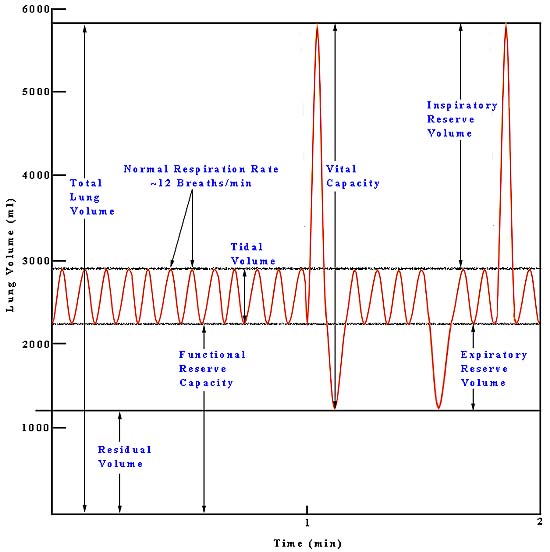
Pulmonary ventilation or breathing is the first step to bringing oxygen to the cells of the body and removing the metabolic waste product, carbon dioxide. Contracting the muscles of the diaphragm results in an inflow of fresh air or inspiration, while relaxation of these muscles or contraction of the abdominals causes expiration of air with the waste product CO2. During normal respiration, the lungs exchange about 500 ml of air 12 times a minute. This is the tidal volume of air inspired or expired. In young adult males, there is an inspiratory reserve volume of about 3000 ml that can be inspired above the tidal volume, while the expiratory reserve volume is about 1100 ml, which can be forcefully expired. The vital capacity includes all of the above yielding about 4600 ml. Well-trained athletes may have values 30-40% higher, while females generally have 20-25% less for the quantities listed above. The lungs contain surfactants, which prevent them from totally collapsing and expelling all air, as it requires too much energy to reinflate them from the collapsed state. (This is one of the primary dangers faced by premature babies born before their genes for producing surfactants have turned on. Effectively, they use more energy to breath than they derive from the process of breathing.) The residual volume represents the amount of air that cannot be expelled even by forceful expiration and averages about 1200 ml. The functional residual capacity is the amount of air that remains behind during normal breathing, which amounts to 2300 ml. Below is a diagram showing these capacities and volumes.

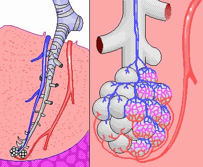
The functioning of the rest of the body depends on an adequate supply of oxygen to the tissues, which depends on respiration through the lungs. There are several respiratory diseases that jeopardize this vital function of the lungs. The respiratory muscles can be damaged by spinal paralysis or poliomyelitis, which can decrease the vital capacity to as low as 500 ml, barely enough to maintain life. The pulmonary compliance reduces vital capacity in diseases like tuberculosis, emphysema, chronic asthma, lung cancer, chronic bronchitis, cystic fibrosis, or fibrotic pleurisy. Several of the diseases above and heart disease can cause pulmonary edema, which decreases vital capacity from fluid build up in the lungs. The alveoli, which are the ends of the branches in the lungs, are where the oxygen actually enters the blood. When the alveoli are damaged or filled with fluid (one result of smoking), the exchange of oxygen is inhibited.

The vital capacity and the residual volume are two values that help physiologists determine the health of the pulmonary system, which translates into the ability of an individual to transport oxygen through the lungs to the rest of the body. The vital capacity is easily measured by taking a deep breath and expiring into a spirometer. For some of the diseases, like emphysema, its important to know the tidal volume and the functional residual capacity, to find the average or minute respiratory volume. When the ratio of the tidal volume to the functional residual capacity becomes too low, then there is insufficient exchange of air to maintain adequate supplies of oxygen to the body.
Discrete Model for Breathing
One method for determining the tidal volume and the functional residual capacity is for the subject to breathe a mixture including an inert gas. The subject breathes the mixture until the lungs are essentially filled with this mixture, then the physiologist measures the amount of the inert gas in a series of breaths after the subject is removed from the gas mixture to normal air. The mathematical model for this experiment is a discrete dynamical system.
Professor Bruce Wingerd ran dilution experiments with the inert gas argon (Ar) to determine some characteristics of his subjects' lungs. Argon is a noble gas, so is totally non-reactive. It also happens to be the third most common gas, comprising 0.93% of Earth's atmosphere. (In dry air, ignoring the partial pressure of water in the atmosphere, Nitrogen, N2, makes up 78%, Oxygen, O2, is second with 21%, while CO2 is a distant fourth with 0.03%.) In Professor Wingerd's experiments, the subjects breathed an air mixture that contained 10% Ar until their lungs were essentially full of this mixture. At the beginning of the experiment, the subjects resumed breathing normal air at a normal rate. Below are tables that show the percent of Ar in each of the next six breaths along with the average volume of air in each breath. The tidal volume is given by the average volume of air in each breath.
|
Normal Subject
Tidal Volume = 550 ml |
|
Subject with Emphysema
Tidal Volume = 250 ml | ||||||||||||||||||||||||||||||||
|
|
|
|
From these data, we would like to determine the functional reserve volume for our subjects. These numbers, along with an experiment to determine the vital capacity using a spirometer, would tell a physiologist a great deal about the health of a subject's lungs.
This breathing experiment is a dynamic exchange of gases, which occurs at discrete intervals of time; hence, it can be written as a discrete dynamical model much as we did in the previous section. The mathematical model tracks the concentration of Ar in the lungs at the time when the lungs have completed inspiration and are ready to cycle through another breath. Define the concentration of Ar at the end of the nth inspiration cycle as cn. To find the concentration at the end of the (n + 1)st inspiration cycle, we need to examine what happens in the lungs while exhaling the air in the lungs from the previous cycle and inhaling fresh air from the atmosphere. For simplicity, we assume the gases become well-mixed during this process, which ignores some of the complications caused by the actual physiological structures in the lungs, such as the "anatomical dead space" in the pharynx, trachea, and larger bronchi or weak mixing from slow gas flow in the alveoli. In fact, of the 500 ml of fresh air brought in by inspiration, only about 350 ml reaches the alveoli, which means that there is less than a seventh exchange of gases with a normal breath.
The physiological parameters needed for this model are Vi for the tidal volume (air normally inhaled and exhaled), Vr for the functional residual volume, and g for the concentration of Ar in the atmosphere. Let q = Vi/(Vi + Vr) be the fraction of atmospheric air exchanged in each breath, so Vr/(Vi + Vr) = (1 - q). Upon exhaling, there remains behind the functional residual volume, which contains the amount of Ar given by Vr cn. The inhaled air during this cycle contains the amount of Ar given by Vi g. (Quantities or amounts of Ar are given by the volume times concentration, and it's the amounts that are conserved.) Thus, the amount of Ar in the next breath is given by
To find the concentration in the next breath we divide by the total volume, Vi + Vr. So we find that
The linear discrete dynamical model for breathing follows from above by substituting the value of q into this equation and results in the model below.
Linear Discrete Dynamical Model for Breathing an Inert Gas
cn+1 = (1 - q) cn + q g.
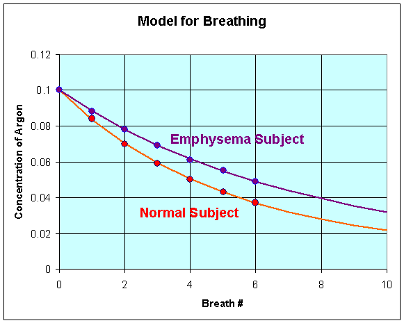
Below is a graph of the data above with the best fitting model for breathing showing both the normal subject and the emphysema patient.

Finding the Functional Reserve Capacity
The object of the experiments above was to find the functional reserve capacity. The diseased states are often characterized by a decreased ratio between the tidal volume and the functional reserve capacity. (Emphysema is characterized by a loss of elasticity in the lungs and a decrease in the alveolar surface/volume ratio.) We can take the discrete dynamical model for breathing an inert gas and readily solve this model for the parameter q. An easy algebraic manipulation gives

From the data for the normal subject, we see that q = (0.1 - 0.084)/(0.1 - 0.0093) = 0.18. The volume of the functional reserve capacity, Vr , is readily found from the formula

By substituting, the data above we find that for the normal subject Vr = 0.82(550)/0.18 = 2500 ml. The ratio of the tidal volume to the functional reserve capacity is 0.22.
A similar analysis of the subject with emphysema gives q = (0.1 - 0.088)/(0.1 - 0.0093) = 0.13. The functional reserve capacity for the subject with emphysema is found to be Vr = 0.87(250)/0.13 = 1670 ml. The ratio of the tidal volume to the functional reserve capacity is 0.15. Notice that this ratio is significantly smaller than the one for the normal subject.
The tables above show the concentration of Ar decreasing in the discrete dynamical model for breathing. If the simulation for the normal individual is carried out for about 3 minutes or 36 breaths, it can be seen that the concentration of Ar drops to 0.0094, which is within 1% of the atmospheric concentration. Since Ar is an inert gas when it comes to breathing, then we expect that after breathing an enriched source of Ar, then eventually the concentration would return to the same value as normally found in the atmosphere. (We are ignoring the fact that H2O makes up a substantial fraction of the air in the lungs as compared to normal air, which is usually much drier.) This value is the equilibrium value of Ar for the model.
Consider a discrete dynamical system given by the equation
where f(xn) is any function describing the dynamics of the model. An equilibrium, xe, for this discrete dynamical system is achieved if xn+1 = xn = xe. That is the dynamic variable settles into a constant value for all n.
In our example above, the mathematical model should reach an equilibrium value that corresponds the the value of Ar in the atmosphere. To find the equilibrium for this model, we substitute
into the discrete dynamical model for breathing. Thus,
which is easily solved and gives ce = g, as expected.
There is an easy way to graphically view the dynamics of these discrete dynamical models. The general model above states that xn+1 = f(xn). Thus, the (n + 1)st state of the model, xn+1, is a function depending on the nth state of the model, xn. We create a graph with the variable xn+1 on the vertical axis and xn on the horizontal axis. We draw the graph of xn+1 = f(xn) and the line xn+1 = xn. A process called cobwebbing allows us to view the dynamics of this discrete dynamical model. We start at some point x0 on the horizontal axis, then go vertically to f(x0) to find x1. Next we go horizontally until we hit the line xn+1 = xn. From here we go vertically to f(x1) to find x2. The process is repeated to give a geometric view of the discrete dynamical model. At any point where the function f(xn) crosses the line xn+1 = xn, there is an equilibrium for the model.
The cobwebbing technique is illustrated with the discrete dynamical model for breathing. Below is a graph showing the simulation for the normal subject listed in the table above.
Notice that for the breathing model, the concentration, cn, tends towards the equilibrium concentration, ce = g. When the solution approaches the equilibrium for large n, then the equilibrium is said to be stable.
Malthusian Growth Models with Immigration or Emigration
In the previous section, we examined the discrete Malthusian growth model for the U. S. population. We saw that a simple Malthusian growth model has a limited value for studying the U. S. population though the nonautonomous Malthusian growth model substantially improved our predictions. These models only account for the net growth of the population in what is considered a closed system, since it acts as if the population is totally dependent on the population being studied. Throughout U. S. history, our population has been significantly affected by the rate of immigration. Through much of the 20th century, the government has regulated legal immigration to 250,000 people per year.
The discrete Malthusian growth model is easily modified to account for either immigration or emigration. Suppose that a population, Pn, grows according to the discrete Malthusian growth model. Assume that a constant number of the population leaves or emigrates in each time interval. The mathematical model for this behavior is given by the equation:
where r is the rate of growth and m is the constant number emigrating. Assuming that the constants are known and if the initial population , P0, is given, then it is easy to determine all subsequent populations by iteration. This model is similar to the breathing model above in that the discrete dynamical model is linear, that is the right hand side of the equation is only a linear function of Pn.
Notice what happens if we attempt to iterate this model starting with P0. We obtain
It is not hard to work the algebra and see that
which simplifies to

This solution is clearly more complicated and harder to obtain than the previous section for the discrete Malthusian growth model. However, few other discrete dynamical models have a solution that can be written as a formula depending only on the parameters, n, and P0, a closed form solution. In the next section, we will study a model with a simple quadratic term on the right side of the equation, yet this discrete dynamical model will have no closed form solution. It can only be simulated one step at a time to determine the exact value of Pn.
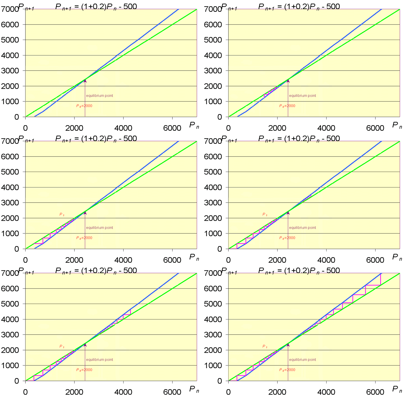
When the solution becomes complicated or impossible to find exactly, then we still would like to obtain some information about the qualitative behavior of the model. The cobwebbing technique illustrated above gives us some ideas on studying the behavior. Below is the cobwebbing diagram for the discrete Malthusian growth model with emigration, where r = 0.2 and m = 500.

The green line represents the model, Pn+1 = 1.2 Pn - 500, while the blue line is what is known as the identity map, Pn+1 = Pn . These lines intersect at the equilibrium point, which solves the equation,
One significant difference between this dynamical model and one for the breathing is that iterations of the solution are going away from the equilibrium. Thus, if the population begins above 2500, then it grows increasingly larger, much like we saw in the previous section for the Malthusian growth model. However, if the population starts below 2500, then more animals leave than can be replaced, so the population is driven to extinction. The equilibrium for the discrete Malthusian growth model with emigration is said to be unstable.
Stability of a Linear Discrete Dynamical Model
The stability of an equilibrium for a Discrete Dynamical Model is important for understanding how that particular mathematical model behaves. Consider the Linear Discrete Dynamical Model given by
yn+1 = a yn + b.
Linear discrete dynamical models have a single unique equilibrium if the slope of the linear function, a, is not 1. (If a = 1, then either there are no equilibria or all points are equilibria (b = 0).) It is easy to see that the equilibrium is given by
![]()
For most modeling situations, the equilibrium (if it exists) must be positive (or zero). It follows that a positive equilibrium exists if either a < 1 and b > 0 or a > 1 and b < 0.
The equilibrium of a linear discrete dynamical
model is stable if either of the following conditions hold:
1. Successive iterations of the model approach the equilibrium.
2. The slope |a| is less than 1.
Similarly, the equilibrium of a linear discrete
dynamical model is unstable if either of the following conditions
hold:
1. Successive iterations of the model move away from the equilibrium.
2. The slope |a| is greater than
1.
A section of Worked Examples is provided to help with the exercises covering this material.
[1] A. C. Guyton and Hall (1997), Textbook of Medical Physiology, W. B. Saunders Co., Philadelphia