Outline of Examples:

1. Algebra of Functions
2. Quadratic Equation
3. Quadratic Functions
4. Applications

Algebra of Functions

Below are a collection of examples that use the definitions and properties of functions developed in the main section.

Example 1: Consider the functions f(t) = t ² - 1 and g(t) = 2 t + 3.

a. Evaluate f(2), f(-1), f(3), g(-2), and g(1).

b. Create the composite functions f(g(t)) and g(f(t)) and write the expressions in the simplest form. Evaluate f(g(1)) and g(f(-1)).

Solution:

a. In the case of f(2) we substitute a 2 for each t in the given equation for f(t) to obtain

Using the above method we obtain the following for f(-1), f(3), g(-2), and g(1)

b. To find f(g(t)) we substitute the entire function g(t) for t into f(t).

By the same method, we obtain the following:

To find f(g(1)), we substitute 1 for t into f(g(t)) to obtain

In an alternate method, we can evaluate g(1) and then substitute this value into f(t) to obtain the same answer, as follows:

From Example 1a, we know that g(1) = 5. Then we must evaluate f(5) to obtain:

Therefore, using either method, g(f(-1)) yields the following result:

Example 2: Use the function f(t) from the previous example.

a. What is the range of this function (assuming a domain of all t)?

b. Find the domain of f(t), if the range of f is restricted to f(t) < 0.

Solution:

a. Recall that f(t) = t² - 1. The domain of f(t), unless otherwise noted, is all real numbers, since any number t substituted into f(t) yields a real, finite answer. However, the range, or output, of the function may not include all real numbers. Graphing the function helps visualize both its domain and range, as shown below.

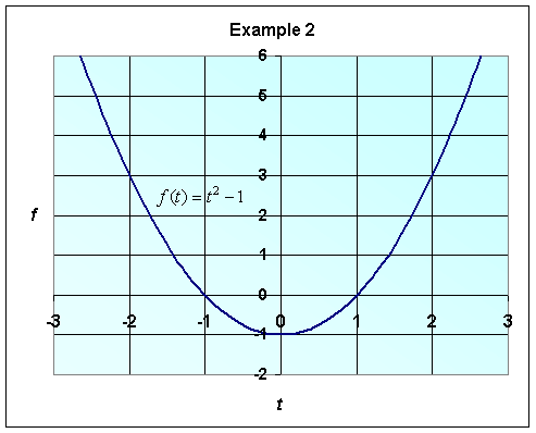
The range of f(t) includes all numbers along the vertical axis for which there is at least one point on the graph. As you can see, the range of the function does not include all real numbers, but does include all numbers greater than or equal to -1. Therefore, the range of f(t) = [-1, ¥) or f(t) > -1.

b. If the range of f(t) is restricted to f(t) < 0, then the domain, which is characterized by all numbers t that can be substituted into the given range of f(t), can also be found by looking at the graph above. Therefore, we can say that for f(t) < 0, the domain includes (-1, 1), or -1 < t < 1. However, the domain cannot always be accurately determined directly from the graph. There following is an alternate method in determining the domain of a function:

We know that f(t) < 0, and that f(t) = t² - 1. Therefore, we can say:

Solving for t, we obtain:

Once again, we find the domain to be -1 < t < 1.

Quadratic Equations

Below are several examples of quadratic equations. These can be solved by either factoring the quadratic or the quadratic equation.

Example 3: Solve the following quadratic equations (if possible):

a. x² - 10x + 16 = 0      b. x² + 2x - 2 = 0      c. x² - 4x + 5 = 0

Solution:

a. The simplest approach this equation is to solve for x by factoring.

Solving for x we find that x = 8 or x = 2.

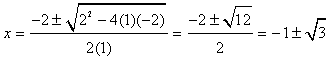
b. This equation does not appear to be easily factorable, so we can resort to using the quadratic formula, as follows:

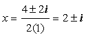
In this case, a = 1, b = 2, and c = -2

c. This equation cannot be solved by factoring, so we use the quadratic formula again, where a = 1, b = -4, and c = 5.

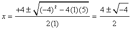
Since we cannot evaluate the square root of a negative number, -4 in this case, there is no real solution for x.

However, there are two complex solutions, where i is the square root of -1, such that:

Quadratic Functions

The example below examines the graphing of a line and a quadratic function.

Example 4: Consider the functions f(x) = x² - 1 and g(x) = 2x + 3. Sketch both of these functions on a single graph. Find the x and y-intercepts for both functions. What is the slope of the line? Find the coordinates of the vertex of the parabola. Finally, determine the coordinates of the points of intersection of these curves.

Solution:

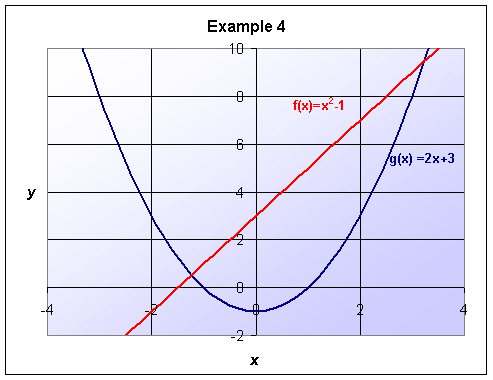
The y-intercept of any function can be found by letting x = 0, and solving for y. To find the x-intercept of a function, one can set y = 0 and solve for x. The intercepts of f(x) are found as follows:

Setting x = 0 for the y-intercept

Letting y = 0 for the x-intercept

So the y-intercept of f(x) is -1, and the x-intercepts are -1 and 1. This means that the graph of f(x) crosses the y axis at -1, and crosses the x axis at -1 and 1, which is consistent with the graph above.

Finding the intercepts of g(x):

For a line of the form y = mx + b, the y-intercept is equal to b; so we can say that for g(x) the y-intercept must be 3. Letting y = 0 for the x-intercept,

x = - or -1.5

Thus, the y-intercept of g(x) is 3, and the x-intercept of g(x)is -1.5, in agreement with the graph above.

Note that the degree of a function, or its highest power, gives the number of possible x-intercepts for the function. This is why f(x) had two solutions for x while g(x) had only one solution.

The slope of g(x) must be m = 2, in accordance with the given slope-intercept form of the line.

The vertex of the parabola f(x) is found from the general form of a quadratic equation:

where the vertex is the point (h, k), and a is a parameter that measures how wide or narrow the curve of the parabola is, as well as in which direction it opens. If a > 0, the parabola is a U-shape which opens upward, and the vertex falls at a minimum. For a < 0, the parabola opens downward, with the vertex as a maximum. In some cases, one must complete the square in order to obtain this form of the quadratic function.

Therefore, for f(x) = x² - 1:

And the vertex is at (h, k) = (0, -1).

Note: There are three methods for finding the vertex: 1. Completing the square. 2. The x-value is x = -b/2a. 3. The midpoint between the x-intercepts.

To find where the two graphs intersect, we first set the two functions equal to each other and solve for x.

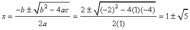
At this point, there are a couple of different methods we can use to solve for x, both of which will yield the same solutions. In this case, we'll use the quadratic formula, where a = 1, b = -2, and c = -4.

~ 3.24, -1.24

Next, we can substitute each of these solutions for x into either equation to find the y coordinates of intersection.

g(x) = ~ 2(3.24) + 3 ~ 9.48

g(x) = ~ 2(-1.24) + 3 ~ 0.52

Therefore, the points of intersection of the two functions are (3.24, 9.48) and (-1.24, 0.52).

Applications

Example 5: A ball is thrown vertically with a velocity of 32 ft/sec from ground level (h = 0). The height of the ball satisfies the equation:

a. Sketch a graph of h(t) vs. t.

b. Find the maximum height of the ball, then determine when the ball hits the ground.

Solution:

a. Note that the function is a relationship between time and the height of the ball. If we start at both time and height equal to zero, the only relevant part of the graph is that which occurs above the x-axis.

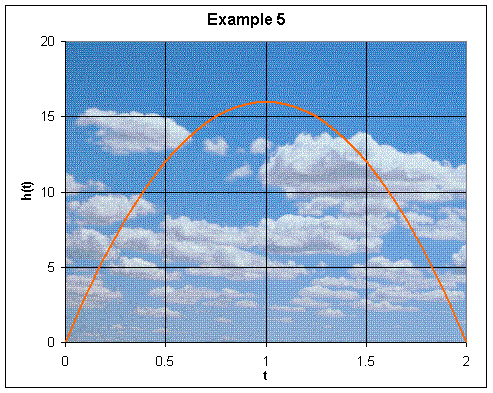
b. Since the graph above shows the height as a function of time, we can see that the maximum height of the ball occurs at the peak of the parabola. Graphically, this appears to be approximately one second after it is thrown into the air, and has a height of somewhere between 15 and 20 feet. A more exact method is to convert h(t) into the general form of a parabola, h(t) = a(t - h)² + k. We can begin by factoring out -16 and then completing the square:

Halving the coefficient of the linear term, we obtain -1. Squaring -1 yields +1. We then both add and subtract this number inside the parentheses (since +1 - 1 = 0 we are not changing anything), and pull out the -1. Be careful to include the -16 that is being multiplied out front when you extract the -1. The reason we keep the +1 inside the parentheses is to make it possible to obtain a perfect square binomial, as in the general equation of the parabola.

Therefore, since the maximum occurs at the vertex (h, k), we know that the ball reached a maximum height of 16 feet one second after it was thrown. Notice that since a is negative, the parabola opens downward, with the vertex at the maximum.

From the graph, the ball appears to hit the ground two seconds after it was thrown. In the algebraic method we set h(t) equal to zero and solve for t.

What we have done is find the x-intercepts of the graph. Since the ball was thrown at time t = 0, we know that the ball hit the ground after two seconds.

Example 6: Use the information in the notes to determine the concentration of [H⁺] for a 1N solution of formic acid. Also, find the pH of this solution.

Solution:

From the lecture notes, we know that K_a = 1.77×10^-4. In this case we are also given that x = 1. The given formula for [H⁺] is as follows:

Using the quadratic formula, we solve for [H⁺] as follows:

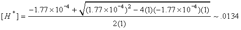
Note that the variable in this quadratic equation is [H⁺], since it has both a quadratic and a linear term. Since it is impossible to obtain a negative amount or concentration of a material, we throw away the negative answer, and keep only that which is positive. Therefore, we have an acid concentration of 0.0134.

The pH is found by -log₁₀[H⁺] = -log₁₀[.0134] ~ 1.87.

Example 7: A spectrophotometer uses the Lambert-Beer law to determine the concentration of a sample (c) based on the absorbance of the sample (A). The ion dichromate forms an orange/yellow that has a maximum absorbance at 350 nm and is often used in oxidation/reduction reactions. The Lambert-Beer law for the concentration of a sample from the absorbance satisfies the linear relationship

where m is the slope of the line.

a. Below are data collected on some known samples

b. Sketch a graph of the data and the line that best fits the data. Then use this model to determine the concentration of two unknown samples that have absorbances of A = 0.45 and 0.62.

Solution:

a. From the lecture, we know how to calculate the sum of squares of the error, as a quadratic function of m:

Expanding and simplifying these terms, we obtain:

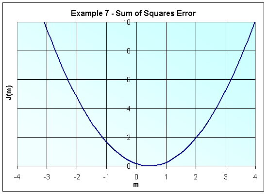
Notice that the vertex of this parabola is not easily obtained graphically. Therefore, we can resort to completing the square of J(m) to obtain the vertex:

Half of the coefficient of the middle term, squared, is (0.8819(.5))² = 0.1944

Therefore, the vertex falls at the point (h, k) = (0.4410, 0.0003).

b. Graphing the linear best fit to the data, we obtain:

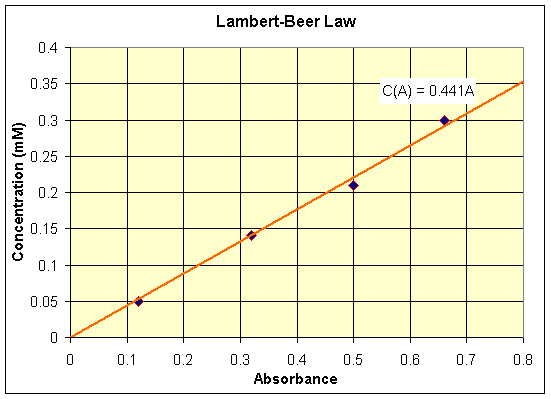
We find the equation of the line to be c(A) = 0.441A through methods described in the Least Squares lecture section. For an absorbance A = 0.45 or 0.62, we simply plug this value into the best fit line to obtain the concentration:

Therefore, for absorbances of 0.45 and 0.62, our model predicts concentrations of 0.198 and 0.273, respectively.