1. Pollution of a Lake Revisited
2. Euler's Method
3. Improved Euler's Method
4. Numerical Solution of the Lake Problem
5. Problems

Pollution of a Lake Revisited

In the last section, we examined how to develop and solve a model based on agricultural runoff of a pesticide into a lake. The model used some very simplistic assumptions, which allowed us to solve the differential equation. In this section we will develop some numerical methods for solving differential equations that allow us to consider more realistic models for pollution of a lake.

One of the leading problems facing the environment today is the very difficult task of removing non-point source pollutants from our water supplies. As a motivating example, we extend the problem from the previous section on the clean up of a pollutant from a non-point source, such as agricultural runoff of pesticide. Suppose that a pesticide that has been used extensively on agricultural fields is found to cause cancer, so is removed from the market. However, if this pesticide does not degrade readily, then it can have a long term lingering effect on the quality of water downstream from the agricultural fields.

Let us develop a more realistic model for this situation. In our modeling scenario this time, the lake is already polluted with the dangerous pesticide. Thus, the concentration in the lake begins at some level, c(0) = c₀. We will still assume that the lake maintains a constant volume V, but suppose that we take into account the seasonal flow of the rivers entering and leaving the lake. Thus, the flow rate, f(t), will be time varying rather than constant as in the last example. For example, if the flow rate varies annually in a sinusoidal manner with a maximum of about 150 m³/day and a minimum of about 50 m³/day, then we can write the flow rate

Even if the pesticide is banned, so that it is no longer being applied to the fields, there remains residual pesticide from the past applications that leaches into the runoff water. Thus, the concentration of the pesticide in the river would be time varying or p(t). Typically, this effect would show an exponential decay after the use of the pesticide is stopped. Much like the radioactive decay problem discussed in the previous section, we might expect the concentration in the runoff water to be proportional to the amount remaining, which would be approximated by a decaying exponential. For example, we might assume that the concentration of the pesticide in the river satisfies

The method to set up the mathematical model for the concentration of the pesticide in the lake, c(t), is exactly the same as developed in the previous section. The differential equation is set up using the mass balance of the pollutant, so

Again the amount entering is the concentration of the pollutant in the river times the flow rate of the river. Thus, f(t) p(t) gives us the amount of pesticide entering the lake per unit time, which is now a time varying function. The amount leaving has the same flow rate, f(t). Since the lake is assumed to be well-mixed, the amount of pollutant leaving the lake per unit time is the product of the concentration in the outflowing river, which equals the concentration of the pollutant in the lake, c(t), times the flow rate f(t). Thus, if a(t) is the amount of pollutant in the lake at any time t, then a differential equation describing a(t) is given by:

As in the previous section, we want a differential equation describing the concentration of the pollutant in the lake with c(t) = a(t)/V. Since we are assuming a constant volume, this implies that c'(t) = a'(t)/V. The above differential equation can be written

If as in the previous section, we assume that the volume of the lake is 10,000 m³ and if the initial level of pollutant in the lake is c₀ = 5 ppm, then using the specific functions listed above we have the initial value problem,

This differential equation is more complicated than any of the examples of the previous section. Though there exist methods for finding an exact solution to this differential equation (since it is a linear first order equation), a good method for approximating the solution is to use a numerical technique for solving differential equations. At the end of this section, we present a numerical solution to this problem.

Euler's Method

Many differential equations do not have an exact solution or they are very complicated, so finding an exact solution is very difficult. In this section, we develop a numerical technique for solving ordinary differential equations. Recall from our introduction to differential equations, we developed the continuous Malthusian growth model from the discrete Malthusian growth model. The idea connecting these two models was the definition of the derivative.

Let us consider a general initial value problem given by the following;

From the definition of the derivative, we can write

Suppose that we don't take the limit, but use a fixed stepsize h. Then an approximation to the derivative is easily seen to be

If we substitute this into the differential equation above, then multiply by h and bring the y(t) to the right hand side, we obtain the approximation to the differential equation given by the formula

Notice that this is very similar to the discrete dynamical systems that we have studied before.

Euler's Method is based on this formula above. This method is what is known as a fixed step method for solving differential equations. Geometrically, Euler's method looks at the slope of the tangent line to the approximate solution at each time step, then proceeds forward one time step to obtain the next approximation to the solution. The ability of this method to track the solution accurately depends on the length of the time step and the nature of the function f(t, y). In practice, this technique is rarely used as it has very bad convergence properties to the actual solution, but it should be easy to understand by its connection to the definition of the derivative.

For Euler's Method we begin by letting y(t₀) = y₀. Let t_n+1 = t_n + h and define the approximation of y(t_n) as y_n. Euler's Method becomes the discrete dynamical system

Example 1:

Let us begin with a Malthusian growth model to explore Euler's Method. Consider the model

 The solution of this problem is P(t) = 50 e^0.2t. Let us approximate this solution on the interval [0,1] using a stepsize of h = 0.1, and compare the approximate solution to the actual solution.

x	Euler Solution	Actual Solution
0	50.000	50.000
0.1	51.000	51.010
0.2	52.020	52.041
0.3	53.060	53.092
0.4	54.122	54.164
0.5	55.204	55.259
0.6	56.308	56.375
0.7	57.434	57.514
0.8	58.583	58.676
0.9	59.755	59.861
1	60.950	61.070

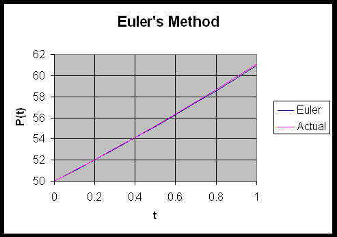
A graph of these solutions is seen in the following.

 

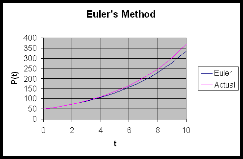
From the table and the graph you can see that Euler's method is tracking the solution fairly well over the interval of simulation. However, this is a fairly short period of time and the stepsize is relatively small. What happens when the stepsize is increased and the interval of time being considered is larger. Below we show a simulation over a time period of 10 using a stepsize of h = 0.5.

Already at this point there is a 9% error in the numerical solution as compared to the actual solution.

Example 2:

In this example, we go through the detailed steps of Euler's method for a differential equation, where the function f(t,y) has both variables appearing. Consider the initial value problem

Suppose you want to find the approximate solution at t = 1, using a stepsize of h = 0.25.

The reader can check to see that the actual solution is y(t) = 4e^t - t - 1. From the information above,we see that Euler's formula for this problem is given by

The easiest way to work Euler's method is to create a table of values where the first column gives the values for t_n and the second column gives the computed values for y_n. Below is a table with the necessary calculations.

tn	Euler solution yn
t0 = 0	y0 = 3
t1 = 0.25	y1 = y0 + h(y0 + t0 ) = 3 + 0.25(3 + 0) = 3.75
t2 = 0.5	y2 = y1 + h(y1 + t1 ) = 3.75 + 0.25(3.75 + 0.25) = 4.75
t3 = 0.75	y3 = y2 + h(y2 + t2 ) = 4.75 + 0.25(4.75 + 0.5) = 6.0625
t4 = 1	y4 = y3 + h(y3 + t3 ) = 6.0625 + 0.25( 6.0625 + 0.75) = 7.7656

Notice that y₄ corresponds to the approximate solution of y(1). The actual solution gives y(1) = 8.87312, so the Euler approximation with this large of a stepsize is not a very good approximation to the actual solution with a 12.5% error. If the stepsize is reduced to h = 0.1, then Euler's method requires 10 steps to find an approximate solution for y(1). It can be shown that y(1) @ y₁₀ = 8.37497, which is better, but still has a 5.6% error.

Improved Euler's Method

As noted above, Euler's method is a simple technique for understanding the connection between differential equations and their numerical solutions. However, we also noted that it does not do a very good job of tracking the solution to the differential equation. There are many numerical methods for solving differential equations with some of them being very accurate. These numerical methods can be used through such standard software as Maple or MatLab. Some of the best are a class of single step methods called Runge-Kutta methods. The simplest of these is called the Improved Euler's method. The formula for this method is given below. It is beyond the scope of this course to show why this technique is significantly better than the Euler's method listed above.

As we did for Euler's Method, we begin by letting y(t₀) = y₀ and define t_n+1 = t_n + h and the approximation of y(t_n) as y_n. The Improved Euler's method uses an average of the Euler's method and an Euler's method approximation to the function. We first need to approximate y by Euler's method, so define

The Improved Euler's formula starts with y(t₀) = y₀ and becomes the discrete dynamical system

.

Example 3:

We return to Example 2 with the initial value problem

To show the difference between Euler's method and Improved Euler's method we create a table of the numerical solution for the differential equation above along with the actual solution, using a stepsize of h = 0.1.

t	Euler's Method	Improved Euler	Actual
0	y0 = 3	y0 = 3	y(0) = 3
0.1	y1 = 3.3	y1 = 3.32	y(0.1) = 3.3207
0.2	y2 = 3.64	y2 = 3.6841	y(0.2) = 3.6856
0.3	y3 = 4.024	y3 = 4.0969	y(0.3) = 4.0994
0.4	y4 = 4.4564	y4 = 4.5636	y(0.4) = 4.5673
0.5	y5 = 4.9420	y5 = 5.0898	y(0.5) = 5.0949
0.6	y6 = 5.4862	y6 = 5.6817	y(0.6) = 5.6885
0.7	y7 = 6.0949	y7 = 6.3463	y(0.7) = 6.3550
0.8	y8 = 6.7744	y8 = 7.0912	y(0.8) = 7.1022
0.9	y9 = 7.5318	y9 = 7.9247	y(0.9) = 7.9384
1	y10 = 8.3750	y10 = 8.8563	y(1) = 8.8731

It is very clear that the Improved Euler's method does a substantially better job of tracking the actual solution. Notice that the error is less than 0.2% when compared to the actual solution at t = 1.

Numerical Solution of the Lake Problem:

At the beginning of this section, we proposed a more complicated model for pollution entering a lake. Our model included an oscillatory flow rate and an exponentially falling concentration of the pollutant entering the lake via the river. The initial value problem was

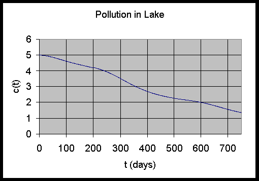
This differential equation is easily solved using either numerical method, while it would be very challenging to solve exactly. A simulation of the model was done using both Euler's method and Improved Euler's method with a stepsize of h = 1, simulating for 750 days (a little over two years). The two solutions could not be distinguished on a graph, so only the result from the Improved Euler's method is graphed below.

This solution shows a much more complicated behavior for the dynamics of the pollutant concentration in the lake. Could you have predicted this behavior or determined quantitative results, such as when the pollution level dropped below 2 ppm? This is much more typical of what we might expect from more realistic biological problems. Thus, the numerical methods allow the examination of more complex situations, which allows the scientist to consider more options in probing a given situation. You should think on how you might want to modify the example above to explore better ways to remove a toxic substance. Numerical simulations allow one to project how different strategies can impact the environment without actually effecting the environment. Still the numerical simulation is only as good as the data entered, so the biologist must carefully measure the inputs to the model, then test it under experimental conditions to gain some sense of reliability.

 Problems:

1. Consider the following initial value problems:

a. y ' = 0.3y, y(0) = 20.

b. y ' = 10 - 0.3y, y(0) = 10.

Solve each of these initial value problems. Next use Euler's method to approximate the solution using a stepsize of h = 0.2. Find the approximate solution for y(1), which uses 5 steps, then compute the error between the actual solution and the approximate solution using Euler's method.

 2. A population of animals that includes emigration satisfies the differential equation

where k = 0.1 and m = 2.

a. Solve this differential equation and find P(1).

b. Use Euler's method with h = 0.2 to approximate the solution at t = 1. Find the percent error between the actual solution and this approximate solution at t = 1.

3. The body temperature of a particular animal is normally 40^oC. Suppose this animal is hit by a car at midnight ( t = 0 ), and the environmental temperature, T_e(t), over the next few hours is slowly decreasing with T_e(t) = 15 - t. From Newton's Law of Cooling, the temperature of the roadkill satisfies the differential equation