Logistic Growth - Worked Examples

 

Example 1 (Logistic Growth model): Consider the logistic growth model given by the equation

p_n+1 = 1.2p_n - 0.0004p_n²,

where n is measured in weeks. Assume that p₀ = 200 and find the population for the next three weeks, p₁, p₂, and p₃.

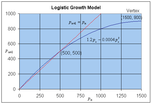
Find all equilibria for this model. Sketch a graph of the updating function (the right hand side of the equation above) along with the line p_n+1 = p_n, showing clearly on the graph the equilibria and the vertex of the parabola.

Solution:

To find the populations for the next three weeks, we begin by substituting the given value for p₀ into the growth model equation.

p₁ = 1.2p₀ - 0.0004p₀² = 1.2(200) - 0.0004(200)² = 224

p₂ = 1.2(224) - .0004(224)² = 248.7

p₃ = 1.2(248.7) - 0.0004(248.7)² = 273.7

From the lecture, we know that p_e = 0 (the trivial solution), or p_e = M. At equilibrium points the above model is

p_e = 1.2p_e - 0.0004p_e²

-0.2p_e + 0.0004p_e² = 0

p_e(0.0004p_e - 0.2) = 0

Thus, the equilibrium points occur at p_e = 0 or p_e = 0.2/0.0004 = 500.

Below is a graph of the updating function, showing the vertex of the parabola and the points of intersection of the updating function with the identity function, which gives the equilibria (one being the origin, not labeled).

 

Example 2 (Growth Rate function): An alternate way to look at discrete population growth models is to consider the population at the (n+1)^st generation as being equal to the population at the n^th generation plus the growth of the population, g(p_n), between the generations. Consider the logistic growth model given by the equation

p_n+1 = p_n + g(p_n) = p_n + 0.05 p_n (1 - 0.0001p_n),

where n is measured in hours. The equilibria can be readily found by determining when the growth rate is zero.

a. Assume that p₀ = 500 and find the population for the next three hours, p₁, p₂, and p₃.

b. Find the p -intercepts and the vertex for

g(p) = 0.05 p(1 - 0.0001p).

Sketch a graph of g(p).

c. By finding when the growth rate is zero, determine all equilibria for this model.

Solution: a. We find the first three iterations by substituting each successive value into the given updating function. Thus,

p₁ = p₀ + g(p₀) = 500 + 0.05(500)(1 - 0.0001(500)) = 524,

p₂ = 524 + 0.05(524)(1 - 0.0001(524)) = 549,

p₃ = 549 + 0.05(549)(1 - 0.0001(549)) = 574.

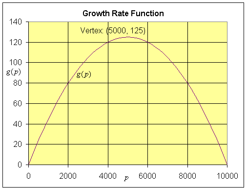
b. Since g(p) = 0.05 p(1 - 0.0001p), the p-intercepts are found by solving g(p) = 0.05 p(1 - 0.0001p) = 0, which gives either p = 0 or 1 - 0.0001p = 0. The latter is equivalent to p = 10,000. The vertex occurs halfway between the p-intercepts, so p = 5,000 and g(5000) = 0.05(5000)(1 - 0.0001(5000)) = 125.

The graph of g(p) is a standard parabola, which is shown below showing the p-intercepts and the vertex.

c. From the graph above, it is clear that the growth rate is zero at 0 and 10,000, so the equilibria occur at p_e = 0 and 10,000.

 

Example 3 (Logistic Growth with Emigration): We extend the previous example to include the possibility that the population might be affected by immigration or emigration. Suppose that the growth rate for a population is given by

g(p) = 0.71 p - 0.001p² - 7.

This says that between each generation there is a 71% growth rate, while 0.001p_n² are lost due to crowding and 7 emigrate. The discrete dynamical model for this population model is given by

p_n+1 = p_n + g(p_n) = p_n + 0.71 p_n - 0.001p_n² - 7,

where n is measured in generations.

a. Assume that p₀ = 100 and find the population for the next three generations, p₁, p₂, and p₃.

b. Find the p -intercepts and the vertex for g(p) and sketch a graph of g(p).

c. By finding when the growth rate is zero, determine all equilibria for this model.

Solution: a. As we did in the previous example, we iterate this discrete logistic model with emigration to obtain the next three generations. Thus,

p₁ = p₀ + g(p₀) = 100 + 0.71(100) - 0.001(100)² - 7 = 154,

p₂ = 154 + 0.71(154) - 0.001(154)² - 7 = 233,

p₃ = 233 + 0.71(233) - 0.001(233)² - 7 = 337.

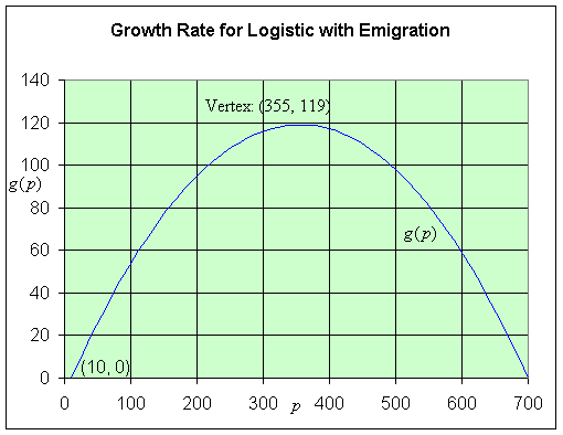
b. Since g(p) = 0.71 p - 0.001p² - 7 = -0.001(p² - 710p + 7000), the p-intercepts are found by solving g(p) = -0.001(p² - 710p + 7000) = -0.001(p - 10)(p - 700) = 0, which gives either p = 0 or p = 700. The vertex occurs halfway between the p-intercepts, so p = 355 and g(355) = -0.001(345)(-345) = 119.

The graph of g(p) is a parabola, which is shown below showing the p-intercepts at p = 10 and 700 and the vertex.

c. From the graph above, it is clear that the growth rate is zero at 10 and 700, so the equilibria occur at p_e = 10 and 700.

 

Example 4 (Hassell's model): There is no reason that the discrete dynamical model should have a quadratic form and in fact, because a quadratic function goes negative for large values of p, this model becomes very unrealistic. Hassell modified this growth model (especially for insect populations) to use a rational function response (a rational updating function).

Consider the discrete dynamical model given by the equation

 

where n is measured in generations.

a. Assume that p₀ = 200 and find the population for the next four generations, p₁, p₂, p₃, and p₄.

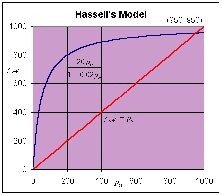
b. Find the p -intercepts and the horizontal asymptote for H(p) and sketch a graph of H(p) for p > 0. (Note that the vertical asymptote occurs at p = -50, which is outside the biologically valid range as p should be greater than or equal to 0.)

c. By solving p_e = H(p_e), determine all equilibria, p_e, for this model.

Solution: a. Once again, we iterate this nonlinear dynamical model by Hassell by substituting the value of p₀ = 200 into the model. The result is

b. The only intercept for H(p) is (0, 0), while the horizontal asymptote is H = 1000. Below is a graph of Hassell's updating function along with the identity map. The intersections give the equilibria.

c. The equilibria are found by setting p_e = p_n+1 = p_n, so we solve

One solution is clearly p_e = 0. Next we multiply both sides by (1 + 0.02 p_e)/p_e, which gives

1 + 0.02 p_e = 20.

Solving this equation gives the other equilibrium, p_e = 950.