Math 121 - Calculus for Biology I Spring Semester, 2001 Applications of the Derivative - Examples
	© 2001, All Rights Reserved, SDSU & Joseph M. Mahaffy San Diego State University -- This page last updated 30-May-01

1. Examples for Stability of the Logistic Growth Model
2. Stability of the Malthusian Growth Model
3. Graphing Polynomials

This section provides a series of examples to supplement the lecture section and help with the homework problems. We also include the Malthusian growth model to see how this analysis applies to this discrete dynamical model.The first examples examine the change in behavior of the nonzero equilibrium of the logistic growth model. The last set of examples looks at more graphing problems.

Examples for Stability of the Logistic Growth Model

Example 1: Consider the discrete logistic growth model given by the equation

Find all the equilibria for this model and use the results from the lecture section to determine the behavior of the solution near these equilibria.

Solution: To find the equilibria, we simply substitute P_e for P_n and P_n+1 into the discrete logistic growth model. This gives

To determine the behavior of the model near the equilibria P_e = 0 and 3000, we need to compute the derivative of f₁(P_e). This is easily done using the power rule, so

To find the behavior near P_e = 0 , we compute f₁'(0) = 1.3 > 1. Thus, the solution monotonically grows away from this equilibrium, which is what we expect.

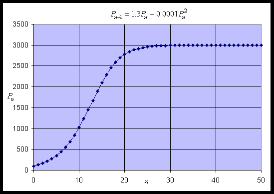
At the other equilibrium, P_e = 3000, we find f₁'(3000) = 1.3 - 0.6 = 0.7 < 1. Thus, from the lecture notes, we see that solutions of the discrete logistic model monotonically approach this equilibrium. This equilibrium is said to be stable. Below we show a simulation of this model, starting with an initial value of P₀ = 100 and performing 50 iterations. The simulation shows the solution growing away from P_e = 0 and approaching P_e = 3000 monotonically.

 

Example 2: We modify the example above slightly and consider the discrete logistic growth model given by the equation

Find all the equilibria for this model and use the results from the lecture section to determine the behavior of the solution near these equilibria.

Solution: As in the previous example, we substitute P_e for P_n and P_n+1 into the discrete logistic growth model giving

The behavior of the model near the equilibria P_e = 0 and 17000 is found by computing the derivative of f₂(P_e). The derivative is given by

At P_e = 0, the derivative is f₂'(0) = 2.7 > 1. Thus, the solution monotonically grows away from this equilibrium.

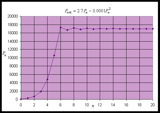
At the other equilibrium, P_e = 17000, the derivative is f₂'(17000) = 2.7 - 3.4 = -0.7. Since -1 < f₂'(17000) < 0, the discrete logistic model oscillates and approaches this equilibrium. This equilibrium is also stable. Below we show a simulation of this model, starting with an initial value of P₀ = 100 and performing 20 iterations. The simulation shows the solution growing away from P_e = 0, then oscillates and rapidly approaches P_e = 17000.

 

Example 3: Another change in the discrete logistic growth model gives the equation

Find all the equilibria for this model and use the results from the lecture section to determine the behavior of the solution near these equilibria.

Solution: As in the previous two examples, we substitute P_e for P_n and P_n+1 into the discrete logistic growth model giving

The behavior of the model near the equilibria P_e = 0 and 22000 is found by computing the derivative of f₃(P_e). The derivative satisfies

At P_e = 0, the derivative is f₃'(0) = 3.2 > 1. Thus, the solution monotonically grows away from P_e = 0.

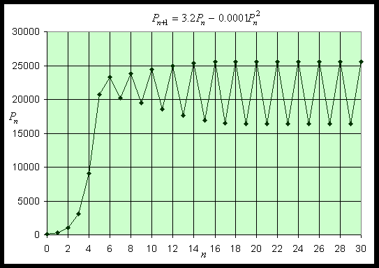
At the other equilibrium, P_e = 22000, the derivative is f₃'(22000) = 3.2 - 4.4 = -1.2. Since f₂'(17000) < -1, the discrete logistic model oscillates and moves away from this equilibrium. Thus, this equilibrium is unstable. Below we show a simulation of this model, starting with an initial value of P₀ = 100 and performing 30 iterations. The simulation shows the solution growing away from P_e = 0, then it settles into a period 2 oscillation taking on the values 16417 and 25583.

 

Example for Stability of the Malthusian Growth Model: The discrete Malthusian growth model was substantially easier to study than the logistic growth model. Its solution was simply an exponentially growing solution. Use the results from the lecture section to show that the only equilibrium of the Malthusian growth model is unstable.

Solution: We assume that there is a positive growth rate for a population of animals satisfying according to the discrete Malthusian growth model, so r > 0. The general Malthusian growth model is given by

The equilibrium is readily found by substituting P_e for P_n and P_n+1, giving

Thus, the only equilibrium for the discrete Malthusian growth model is the trivial solution, P_e = 0. When we take the derivative of the right hand side of the model, we find that the derivative is (1 + r), which is greater than one. This means that for any positive growth rate, the discrete Malthusian growth model is unstable, and the solution monotonically moves away from the equilibrium. This is in agreement with the exponential growing behavior shown earlier.

Examples of Graphing Problems: Below are two more examples of graphing problems, where we can apply the derivative and second derivative to help with the sketch of the graph.

Example 5: Use the techniques developed in lecture to find the minima, maxima, and points of inflection for the following polynomial:

Sketch a graph of the function.

Solution: When you want to sketch a graph, the most important part of sketching the graph is finding the extrema (maxima and minima). These are found by finding the derivative and setting it equal to zero. The solutions of the equation for the derivative equal to zero give the critical values, which are substituted back into the the original function. By adding the x and y-intercepts (if possible) and any asymptotes (if they exist) to the sketch, you can get a fairly good idea of what the graph looks like. The second derivative provides nice information to aid with the graph, but it's not nearly as essential in getting a good looking graph.

The y-intercept should always be easy, and in this case, we readily see that (0, 0) is both an x and y-intercept. We can factor this equation and solve for the x-intercept. To find the x-intercept, set y = 0, then factor and solve the equation,

To find the extrema, we take the first derivative of the function and set it equal to zero. Then we solve for x_c, where y' = 0.

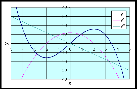
We evaluate the original function at the critical points, giving y(-2) = -16 and y(2) = 16, so the critical points of the function are (-2, -16) and (2, 16). Clearly, the first point is a minimum and the second is a maximum. However, we can check this with the second derivative test. We take the second derivative and evaluate at the critical points to see if they are minima or maxima.

Thus the point (-2, -16) is a local minimum and the point (2, 16) is a local maximum. The points of inflection occur at the point where the second derivative is equal to zero. In this case, the inflection point is at x = 0. This means that the concavity direction changes at point (0, 0). The concavity is upward to the left of (0, 0), and downward to the right of (0, 0). The graph below shows the function and its first and second derivatives.

Example 6: Use the techniques developed in lecture to find the minima, maxima, and points of inflection for the following polynomial:

Sketch a graph of the function.

Solution: See the discussion in Example 5 about the most important steps in sketching a graph. The order of importance are: 1. Find any x or y - intercepts. 2. Find any asymptotes. 3. Find extrema (minima and maxima). 4. Find any points of inflection.

The y-intercept is easily found as (0, 0), which is both an x and y-intercept. We can factor the equation above and solve for the x-intercept

The critical points x_c can be found when the first derivative of the function is set equal to zero.

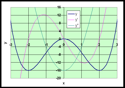
The critical points are at x_c = -2, 0, 2. As before, we evaluate the function at each of the critical points, y(-2) = -16, y(0) = 0, and y(2) = -16, so the critical points of the function are (-2, -16), (0, 0), and (2, -16). Clearly, the first point is a minimum, the second is a maximum, and the third is a minimum again.

Again we can check with the second derivative (though I rarely do so, as it's mostly an exercise dreamed by mathematicians to get students to take more derivatives). The nature of these critical points can be found by evaluating the second derivative function at the critical points of the first derivative function. If the result is negative it indicates a maximum and if the result is positive it indicates a minimum.

Thus the critical points indicate local minima at (±2,-16) and a local maximum at (0, 0). The inflection points occur at the zeros of the second derivative function, which are at approximately (±1.155, -8.889). These characteristics are illustrated in the graph below.