|
|
Math 121 - Calculus for Biology I |
|
|---|---|---|
|
|
San Diego State University -- This page last updated 29-Dec-01 |
|
|
|
Math 121 - Calculus for Biology I |
|
|---|---|---|
|
|
San Diego State University -- This page last updated 29-Dec-01 |
|
![]()
The first sections examined linear models and how to find the best linear model from a set of data. Biological problems are rarely linear, so this section will begin our study of other functions. We will give the mathematical definitions needed to study more general functions, then review quadratic functions.
Our opening example is a linear model from the study of Escherichia coli. However, to fit the data to this model using the least squares best estimate, quadratic functions are needed.
The last section began with a discussion of the DNA replication cycle in E. coli. DNA provides the genetic code for all of the proteins, which are used either directly or indirectly for all aspects of the growth, maintenance, and reproduction of the cell. The synthesis of proteins follows the processes of transcription and translation.
Transcription of a bacterial gene is a controlled sequence of steps, where the protein, RNA polymerase, reads the genetic code and produces a complementary messenger RNA (mRNA) template. This mRNA is a short-lived blueprint for the production of a specific protein that has some particular activity in the bacterial cell.
Translation of the mRNA in bacteria begins shortly after transcription starts, with ribosomes (consisting of ribosomal RNA and ribosomal proteins) reading the triplet codons on the mRNA. The ribosome sequentially assembles a series of amino acids (based on the specific codons read), which form a polypeptide. It is believed that the physical properties of the atoms in the polypeptide cause it to fold passively into a tertiary structure that either becomes an active protein or, when combined with other elements from the cell (such as another polypeptide or lipids), becomes an active protein or enzyme.
The rate of growth of a bacterial cell depends on the rate at which it assembles all of the components inside the cell. However, the rate of production of different components inside the cell varies depending on the length of time it takes for a cell to double. The table below shows the doublings/hr, denoted m, and the rate of mRNA synthesis/cell, denoted rm.
|
|
|
|
|
|
|
|
|
|
|
|
|
|
Due to the instability of the mRNA, its rate of production closely approximates the rate of growth of a cell. The data are seen to lie almost on a straight line passing through the origin, which suggests a linear mathematical model of the form
for some value of a, which is the slope of the linear model.
A linear least squares best fit of this model to the data above can be used to find the slope of the model, a. The sum of the squares of the errors is computed using the formula from the previous section. From the data above and the model, we find each of the error terms as follows:
We expand each of these squared terms and add them together. The resulting equation is
where J(a) is a quadratic function representing the sum of the squares of the errors. As noted in the previous section, the best fit of the model is found by finding the smallest value of J(a), which is the vertex of this quadratic equation.
Below is an applet, where on the left you can manipulate the slope, a, of the line to fit the data (as before), while on the right you observe the value of the quadratic function, J(a). Notice that the best fit to the data occurs at the vertex of the parabola traced by J(a). The vertex of the parabola above is (a, J(a)) = (9.14, 2.45).
Below we use this example to illustrate some fundamental ideas that we use in this course about functions.
Definitions and Properties of Functions
Functions form the basis for most of this course. Simply put, a function is a relationship between one set of objects and another set of objects with only one possible association in the second set for each member of the first set. We have two functions in our example above. The first function has a set of possible cell doubling times, m, to which was found a particular average rate of mRNA synthesis, rm. (You can focus on either the experimental data, which represents a function with a finite set of points, or the linear model, which creates a different function representing your theoretical expectations.) The sum of the squares of the errors between the data points and the model, J(a), forms another function, where the set of possible slopes, a, in the model, each produced a number, J(a), representing how far away the model was from the true data. We claimed that the best model is when this function is at its lowest point. One application of Calculus is to help determine the lowest or minimum value of a function.
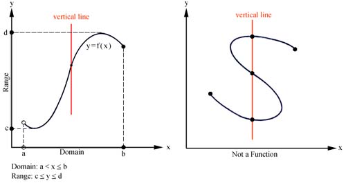
Function: A function of a variable x is a rule f that assigns to each value of x a unique number f(x). The variable x is the independent variable, and the set of values over which x may vary is called the domain of the function. The set of values f(x) over the domain gives the range of the function.
Often we describe a function by using a graph in the xy-coordinate system. By convention we usually let x be the domain of the function and y be the range of the function. The graph is defined by the set of points (x, f(x)) for all x in the domain.
The vertical line test states that a curve in the xy-plane is the graph of a function if and only if each vertical line touches the curve at no more than one point. Below are two graphs showing a function with its domain and range and another graph where the vertical line test shows that it is not a function.
Addition and multiplication of functions are carried out symbolically by standard algebraic techniques. Below we review a couple of examples, which should be familiar from your previous courses in algebra.
Example: Let f(x) = x - 1 and g(x) = x2 + 2x - 3. Determine f(x) + g(x) and f(x)g(x).
Solution: f(x) + g(x) = x - 1 + x2 + 2x - 3 = x2 + 3x - 4.
f(x)g(x) = (x - 1)(x2 + 2x - 3) = x3 + 2x2 -3x - x2 - 2x + 3 = x3 + x2 - 5x + 3.
Example: Determine f(x) + g(x) for
Solution:
Composition of Functions is another important operation. Given functions f(x) and g(x), the composite f(g(x)) is formed by inserting g(x) wherever x appears in f(x). Again this should be review from courses in algebra, so we demonstrate the composition of functions using an example.
Example: Let f(x) = 3x + 2 and g(x) = x2 - 2x + 3. Determine f(g(x)) and g(f(x)).
Solution: f(g(x)) = 3( x2 - 2x + 3) + 2 = 3x2 - 6x + 11, while
g(f(x)) = (3x + 2)2 - 2(3x + 2) + 3 = 9x2 + 6x + 3.
More Worked Examples are provided on a hyperlinked page.
Quadratic Equations and Quadratic Functions
After straight lines, the next easiest algebraic functions to analyze are the quadratic functions. You should have studied quadratic equations and the graphing of quadratic functions (parabolas) in your prerequisite algebra course. The example below shows a classic problem in Chemistry that requires the use of the quadratic equation.
Many of the organic acids found in biological applications are weak acids. Also, weak acid chemistry plays an important role when you are preparing buffer solutions to stabilize certain laboratory cultures. Let us review weak acid chemistry and see how the algebra of quadratic equations come into play.
Formic acid (HCOOH) is a relatively strong weak acid that ants use as a defense. (The strength of this acid makes the ants very unpalatable to predators.) The chemistry of dissociation is given by the following equation:
Each acid has a distinct equilibrium constant Ka that depends on the properties of the acid and the temperature of the solution. For formic acid, Ka = 1.77×10⁻⁴. Let [X] denote the concentration of a particular chemical species X, then assuming that the formic acid is in equilibrium, it satisfies the following equation:
If formic acid is added to water, then [H+] = [HCOO-]. Also, if x is the normality of the solution, then x = [HCOOH] + [HCOO-]. (The anion HCOO- must be either in the bound form HCOOH or ionized form HCOO- with the total representing the normality of the formic acid added to solution.) It follows that [HCOOH] = x - [H+]. Thus,
which is a quadratic equation in [H+] and is easily solved using the quadratic formula. The solution is given by
Notice that we only take the positive solution from the quadratic equation to make physical sense.
Example: Find the concentration of [H+] for a 0.1N solution of formic acid.
Solution: Since formic acid has Ka = 1.77×10⁻⁴ and we have a 0.1N solution of formic acid, then we can substitute into the formual given above to yield:

Thus, the concentration of acid in the 0.1 N solution is [H+] = 4.12 ×10⁻³, which gives a pH of 2.385. (Note that pH is defined to be -log10 [H+].)
Quadratic equations are covered in standard courses in algebra. The general quadratic equation is given by the formula:
There are two methods for solving this type of equation: 1. Factoring the equation and 2. The quadratic formula, which has the form
In the example above, we used the quadratic formula because we didn't know either Ka or x. Let us demonstrate each of these techniques with a few examples.
Example 1 (Factoring): Consider the following quadratic equation:
Find the values of x that satisfy this equation.
Solution: The equation above is easily factored to give the solution.
Example 2 (Quadratic formula): Find the roots of the quadratic equation:
Solution: In this case, we apply the quadratic formula, which gives us the solutions
The general form of a quadratic function is
where a is a nonzero constant and b and c are arbitrary. The graph of this function
produces a parabola. Notice that for each value of x, there is only one value of y. However, for most values of y in the range of this function, there are two values of x. (A horizontal line intersects the graph in two places.)
Example: Let us find the intersections of the line y = 3 - 2x and the quadratic function
Sketch a graph of these functions.
Solution: To find the points of intersection, we set the equations equal to each other. Thus,
This equation is easily factored giving
so x = -4 or 3. By computing the y values corresponding to x = -4 and 3, we obtain the points of intersection as (-4, 11) and (3, -3).
Below is a graph of the two functions
More Worked Examples are provided on a hyperlinked page.
[1] H. Bremer and P. P. Dennis, "Modulation of chemical composition and other parameters of the cell by growth rate," Escherichia coli and Salmonella typhimurium, ed. F. C. Neidhardt, American Society of Microbiology, Washington, D.C., 1987.