Lab F4 - Solutions

In 1950, Version 1: France was the 12^th most populous nation, while in 2000, it fell to the 21^st most populous nation Version 2: Japan was the 5^th most populous nation, while in 2000, it fell to the 9^th most populous nation Version 3: Mexico was the 16^th most populous nation, while in 2000, it became the 11^th most populous nation. Using data from the U. S. census bureau, the table below presents the population (in millions) for Version 1: France Version 2: Japan Version 3: Mexico. This lab has you repeat for this country the modeling effort that we performed in class for the U. S.

a. Find the growth rate for each decade with the data above by dividing the population from one decade by the population of the previous decade and subtracting 1 from this ratio. Associate each growth rate with the earlier of the two census dates. Determine the average (mean) growth rate, r, from the data above. Associate t with the earlier of the dates in the growth ratio, and use EXCEL's trendline to find the best straight line

k(t) = a + bt

through the growth data. Graph the constant function r, k(t), and the data as a function of t over the period of the census data. It is very important that you click on the trendline equation and reformat the coefficient b so that it has more significant figures (obtain 4 significant figures for a and b).

b. The Discrete Malthusian growth model is given by

P_n+1 = (1 + r)P_n.

where r is computed in Part a. and P₀ is the population in 1950. Write the general solution to this model, where n is in decades. Use the model to predict the population in 2020 and 2050.

c. The revised growth model is given by

P_n+1 = (1 + k(t_n))P_n.

where k(t_n) is computed in Part a. and P₀ is again the population in 1950. Simulate this nonautonomous discrete dynamical model from 1950 to 2050. (Note that t_n = 1950 + 10n.) Use the model to predict the population in 2020 and 2050.

d. Create a table listing the date, the population data, the predicted values from the Malthusian growth model, the Nonautonomous dynamical model, and the percent error between the actual population and each of the predicted populations from the models from 1950 to 2000. What is the maximum error for each model over this time interval? Use EXCEL to graph the data and the solutions to the each of the models above for the period from 1950 to 2050. Briefly discuss how well these models predict the population over this period. List some strengths and weaknesses of each of the models and how you might obtain a better means of predicting the population.

e. The growth rate of the Nonautonomous dynamical model goes to zero during this century for Version 1: France Version 2: Japan Version 3: Mexico. At this time, this model predicts that the population will reach its maximum and start declining. Use the growth rate k(t) to find when this model predicts a maximum population, then estimate what that maximum population will be.

Solutions:

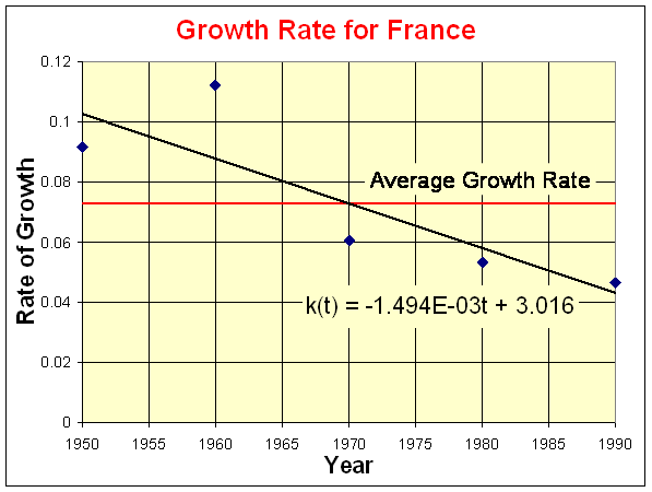
Version 1: a. The table below shows the growth rate per decade for France. The average growth rate for France is given by r = 0.07287, and the best straight line growth rate from the data is given by the formula

k(t) = 3.016 - 0.001494 t.

Year	1950	1960	1970	1980	1990
Growth Rate	0.09180	0.1121	0.06064	0.05328	0.04653

Below is a graph of the growth rate for each decade, which includes the trendline from Excel, the data, and a horizontal line for the average growth rate.

b. The general solution to the discrete Malthusian growth model for France with the average growth rate is given by

P_n = (1.07287)ⁿ41.83.

This model predicts that the population will be P₇ = 68.44 million in 2020 and P₁₀ = 84.52 million in 2050.

c. The nonautonomous discrete dynamical system, which simulates the growth of France's population, is given by

P_n+1 = (4.016 - 0.001494 t_n)P_n, 

where t_n = 1950 + 10n. This model predicts that the population will be P₇ = 61.85 million in 2020 and P₁₀ = 58.77 million in 2050.

d. Below is a table giving the population (in millions) data, the Malthusian growth model (along with its percent error), and the modified Malthusian growth model (along with its error).

Year	Population	Malthusian Model	% Error	Modified Model	% Error
1950	41.83	41.83	0	41.83	0
1960	45.67	44.88	-1.73	46.13	0.998
1970	50.79	48.15	-5.20	50.17	-1.21
1980	53.87	51.66	-4.11	53.83	-0.079
1990	56.74	55.42	-2.32	56.94	0.36
2000	59.38	59.46	0.13	59.39	0.014

The maximum error for the discrete Malthusian growth model occurs in 1970 with the predicted value being 5.2% too low, while the modified Malthusian growth model has a maximum error of -1.21%, also in 1970. Below is a graph of the data and the solutions to the models in Parts b. and c.

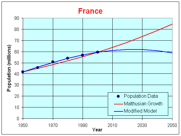
From the error analysis, the nonautonomous Malthusian growth model is better at predicting the actual population and shows only a very small error. Both models predict the population reasonably well since the time interval is fairly short, but as seen in the graph, the nonautonomous Malthusian growth model does extremely well. The main strength of the discrete Malthusian growth model is its simplicity. However, the minor modification of a linear growth rate in the nonautonomous Malthusian growth model substantially increases the accuracy of the model without making the model much more complicated. Both models match the population data fairly well. Their simplicity is also a weakness as it doesn't give one confidence that the model can predict too far into the future. These models give no information about how population is divided into age groups or other important demographic information. There are any number of more complicated models, especially using statistical techniques, that will provide better future predictions. 

e. The growth rate, k(t), is zero when t = 2018.7. Thus, the nonautonomous Malthusian growth model for France predicts that France will achieve its maximum population late in the year 2018. From the simulation, we see that this maximum population should be approximately 61.85 million (the predicted population for 2020).

Version 2: a. The average growth rate for India is given by r = 0.1545, but India's growth rate is actually increasing (opposite the trend in the U.S.). Below is a graph of the growth rate for each decade, which includes the trendline from Excel, the data, and a horizontal line for the average growth rate.

 

b. Below is a table showing the simulation of the discrete Malthusian growth model for India with the average growth rate r = 0.1545. 

Year	Population	Year	Population	Year	Population
1901	238	1941	423	1981	751
1911	275	1951	488	1991	867
1921	317	1961	564	2001	1001
1931	366	1971	651

c. Below is a table with the values for the nonautonomous discrete dynamical system, which simulates the growth of India's population.  

Year	Population	Year	Population	Year	Population
1901	238	1941	321	1981	662
1911	246	1951	370	1991	844
1921	261	1961	438	2001	1102
1931	286	1971	532

d. Below is a graph of the data and the solutions to the models in Parts b. and c.

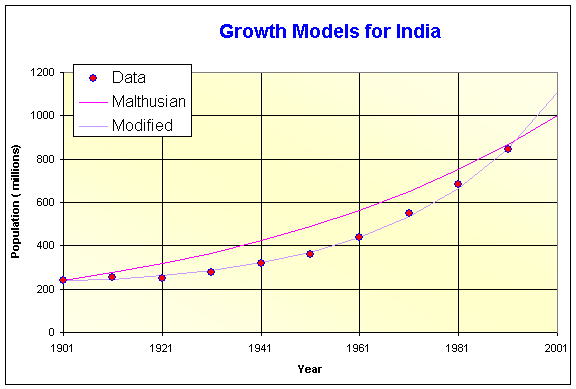
The graph shows the Modified model very closely approximating the population, while the Malthusian growth model fails to predict well through the intermediate range. This is because India's population is accelerating as seen from the growth data in Part a., so the mean population growth poorly represents population trends as we saw in the U.S. population models. The strength in these models is their relatively accurate match to the data, yet they are fairly simple, especially the Modified model. The simplicity of the Malthusian growth model shows its weakness, as fails to match the data in the intermediate range. The Modified growth model should be reasonable for predicting India's growth over the short term, but clearly India cannot keep accelerating its population growth. There are any number of more complicated models, especially using statistical techniques, that will provide better future predictions.

e. Below is a table with the percent errors for the dates 1921, 1961, and 1981 between the data and the Malthusian growth model and the improved nonautonomous growth model. The Improved model shows excellent agreement to the actual data at these dates, while the Malthusian Growth model fails, especially at the intermediate dates.

Year	Malthusian	Modified
1921	26. 4	4.23
1961	28.4	0.26
1981	10.0	-2.48

Below is a table for the predicted populations in 2001 and 2051.

Year	Malthusian	Modified
2001	1001.5	1101.7
2051	2054.3	5824.5

The predicted populations for the Malthusian growth model is probably a bit low, while the Modified Malthusian growth model is probably only slightly high for the 2001 population based on the trends and the graph. The predictions for both models for 2051 are certainly too high. India would be incapable of supporting such high populations, especially the one predicted by the Modified Malthusian growth model. (This prediction would lead to massive starvation or disease that would curtail the population growth.) It is possible, but unlikely that the Malthusian prediction will be close.

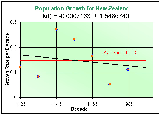
Version 3: a. The average growth rate for New Zealand is given by r = 0.148. Below is a graph of the growth rate for each decade, which includes the trendline from Excel, the data, and a horizontal line for the average growth rate.

b. Below is a table showing the simulation of the discrete Malthusian growth model for New Zealand with the average growth rate r = 0.148. 

Year	Population	Year	Population	Year	Population
1926	1.40	1956	2.12	1986	3.20
1936	1.61	1966	2.43	1996	3.67
1946	1.84	1976	2.79	2006	4.21

c. Below is a table with the values for the nonautonomous discrete dynamical system, which simulates the growth of New Zealand's population.  

Year	Population	Year	Population	Year	Population
1926	1.40	1956	2.20	1986	3.26
1936	1.64	1966	2.52	1996	3.67
1946	1.90	1976	2.87	2006	4.10

d. Below is a graph of the data and the solutions to the models in Parts b. and c.

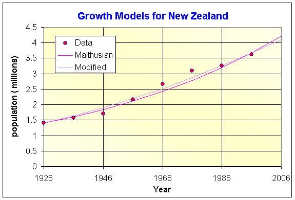
The graph of the two models agree fairly closely through the range of the data, yet show a divergence for future predictions. The extreme fluctuating data in Part a. indicates that neither model will be overly reliable as neither the mean nor a straight line fit through the data should be a good representation. Since the growth data in Part a. showed an almost random pattern about the mean and the trendline was almost flat, one would expect the two models to agree fairly closely, as they do, but the data remains scattered about the models. The strength in these models is their relatively accurate match to the data for their simplicity. Their simplicity is also a weakness as it doesn't give one confidence that the model can predict too far into the future. There are any number of more complicated models, especially using statistical techniques, that will provide better future predictions.

e. Below is a table with the percent errors for the dates 1936, 1966, and 1986 between the data and the Malthusian growth model and the improved nonautonomous growth model. Both the Malthusian and Improved models show excellent agreement to the actual data at these dates.

Year	Malthusian	Modified
1936	2.34	4.25
1966	-8.69	-5.26
1986	-1.86	-0.09

Below is a table for the predicted populations in 2006 and 2056.

Year	Malthusian	Modified
2006	4.21	4.11
2056	8.39	6.54

The predicted population for the Malthusian growth models is slightly high for the 2001, while the Modified Malthusian growth model is probably fairly accurate, based on the trends and the graph. The predictions for both models for 2051 are almost certainly too high for the Malthusian growth model, but the Modified Malthusian growth model is probably not that far off considering the long term prediction. (The trend of the modified growth, k(t), is probably about right.)