Math 636 - Mathematical Modeling Fall Semester, 2007 Allometric Modeling and Dimensional Analysis
	© 2001, All Rights Reserved, SDSU & Joseph M. Mahaffy San Diego State University -- This page last updated 11-Oct-07

Allometric Modeling and Dimensional Analysis

Allometric or Power Law Model

We have seen that using a least squares fit to nonlinear data can be difficult. However, there are a few standard nonlinear models used in biological applications that are more easily analyzed. The technique that we'll develop in this section is known as the Power Law of Modeling. It is also referred to as Allometric Modeling. Allometric models are used regularly in modeling complex biological phenomena where the actual mechanisms underlying the model behavior are too complex to describe in detail, but there is a need to be able to make some predictions.

Allometric models assume a relationship between two sets of data, x and y, that satisfy a power law of the form

where A and r are parameters that are chosen to best fit the data in some sense. Note that this model assumes that when x = 0, then y = 0. As always, you should be aware of the limitations of this type of modeling. This method provides its best predictive capabilities when examining a situation that lies between the given data points. For example, if the number of species of herptofauna on Carribean islands is determined for a collection of islands with varying areas, then this model would give a reasonable estimate for the expected number of species on another Carribean island with an area that lies between the collected data. It would not be appropriate for extending to a large continent as the area is significantly beyond the range of the collected data.(This example is covered in a homework exercise.) It wouldn't even be appropriate for another island such as Iceland, which lies in a different type of climate and has a different geography.

Cumulative AIDS cases

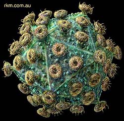
The advent of AIDS in modern society has had a significant impact on both personal behavior and public policy. The new protease inhibitors have significantly improved the quality of life for those who are HIV positive; however, this has come at a substantial cost to society. The new drugs are extremely expensive, are difficult to take because of the complex scheduling requirements to be effective, and have many strong side effects (besides not always working for a particular person or strain of the HIV virus). In turn, there are a number of people who are now avoiding safe sex practices as they no longer fear the "Death Sentence" that used to be associated with an HIV infection. Below is a figure illustrating the HIV virus. It has links to more images with more details about the virus.

	......
..		..
	[click for enlarged and detailed image] illustration by Russell Kightley Media, all rights reserved http://www.rkm.com.au

There is an important need for our society to know the extent of this disease from both an economic and sociological perspective. In order to make informed public policy, we need to know what is the expected case load in the upcoming years. However, it is clearly an extremely complex modeling problem. Below is a table of cumulative cases of AIDS between 1981 and 1992 [2] and an animated .gif showing the spread of the disease (through mortality statistics) over a similar period of time.

Year	Cumulative AIDS Cases (thousands)
1981	97
1982	709
1983	2,698
1984	6,928
1985	15,242
1986	29,944
1987	52,902
1988	83,903
1989	120,612
1990	161,711
1991	206,247
1992	257,085

..		..
	click here to view mpeg

A quick glance at the data will clearly show that it is not linear, so a linear model is not appropriate. There are general methods for finding the least squares best fit to nonlinear data. However, these techniques are very complicated an often difficult to implement. A hyperlink provides an applet for finding the best nonlinear least squares fit to the data for cumulative AIDS cases, which is different from the technique we'll show below.

Allometric models are found by taking the logarithms of the data (or graphing the data on log-log graphs) and seeing if the data lie roughly on a straight line. If this is the case, then a power law relationship makes a reasonable model. Below is an applet showing the linear least squares fit to the logarithms of the data for cumulative aids cases, and the graph to the right shows the modeling relationship with a normal scale. The allometric model has x be time in years since 1980 and y be the cumulative AIDS cases.

The applet above can be adjusted until you reach a minimum least squares for the log of the data with J(A,r) = 0.10. The best slope is r = 3.27 and the best intercept is ln(A) = 4.42. We will show later that this gives the best fit power law for this model as

The graph shows that the power law provides a reasonable fit to the data. Unfortunately, the fit is weakest at the end where we'd like to use the model to predict the cumulative AIDS cases for the next year. The model predicts 366,990 cases in 1993, which is clearly too high from the given data. However, the analysis does give some indication of the rate of growth for this disease, which provides a first approximation for improved models and could be applied to expected spread of another disease with similar infectivity as HIV. This modeling technique is still valuable for analysis of many other data sets and occasionally can provide insight into the underlying biology of the problem. A better fit to the data is shown in the nonlinear least squares appendix that can be viewed through the hyperlink.We will see more examples of this in the computer labs.

Our least squares best fit to the data above uses the logarithms of the data. To detail how the parameters A and r in the model are found, we need to review the properties of exponents and logarithms.

Finding Allometric Models

We return to the Allometric model developed above, where two sets of data, x and y are assumed to satisfy a power law of the form

We want to choose the parameters A and r that best fit the data. The next step is to take the logarithm of both sides, then use the properties of logarithms to simplify the equation.

From this formula, we see that if we take the logarithm of the data, ln(x) and ln(y) and graph it we should see a straight line. That is, if we take X = ln(x), Y = ln(y), and a = ln(A), then the above equation can be written Y = a + rX , which is a line with a slope of r and a Y-intercept of ln(A).

We return to the example at the beginning of this section. Below is a table that includes both the data and the logarithms of the data.

Below shows a graph of the logs of the data (year-1980 and cumulative AIDS cases) along with the best straight line fit.

The plot above shows that when the logarithms of the data for the cumulative AIDS cases are plotted against the logarithms of the time since 1980, then these logarithmic data lie fairly close to a straight line though the data are flattening for the later years suggesting a diminished rate of increase. The least squares best fit of the straight line to the logarithms of the data give a slope of r = 3.274 and intercept of a = ln(A) = 4.415, which gives A = 82.70. Whenever this is the case, then an allometric or power law model makes a reasonable description of the data.

Log-Log Graphs

There exist graphing routines that readily create what is known as a log-log plot. This allows the user to simply graph the data directly onto a graph with logarithmic scales on the axes to see if the data falls on a straight line suggesting an allometric or power law model. Below we show a plot of the original data on cumulative AIDS cases against the date - 1980 on a graph with logarithmic scaled axes.

Example: (Weight and pulse) We know that smaller animals have a higher pulse than larger animals. Let us assume that this relationship satisfies an allometric model. Later in Lab we will perform a more detailed study of this phenomenon to check on the validity of using the allometric model (or power law).

We are given that a 17 g (or .017 kg) mouse has a pulse of 500 beats/min. Assume a 68 kg human has a pulse of 65. Use these data to form an allometric model and predict the pulse for a 1.34 kg rabbit.

Solution: The power law gives

Next we take logarithms to obtain:

As noted above, this is a straight line in ln(P) and ln(w) with slope of k and intercept of ln(A). From the data,

Animal	Weight (kg)	ln(w)	Pulse (beats/min)	ln(P)
Mouse	0.017	-4.075	500	6.215
Human	68	4.220	65	4.174

The slope k is given by:

We can use this slope with one of the points to find ln(A) as follows:

Thus,

If we use the first equation with a 1.34 kg rabbit, then it gives P = 171.

Arguments from Scale

In this section we shall analyze speed of racing shells in rowing using only a similarity analysis [1]. The question that we address is how and why do rowing times vary from class to class. Below is diagrammed a racing shell viewed from above and a cross-sectional diagram.

Insert diagram here.

We shall consider several classes. Eight man lightweight and heavyweight, four man, pairs, and one man scull. In international competition over a 2000 meter course, the heavyweight eight has about a 5% better time than does the lightweight eight. The average heavyweight crew member weighs about 86 kg, while that of the lightweight crew member is only 73 kg. We also have the following table of data from four international races:

Times from four international 2000 m races

We begin by trying to explain the 5% difference between the light and heavyweight crews as they race in almost identical shells. The forces that we need to consider are the power of the oarsmen and the drag of the water. If we assume that the speed is almost constant then we know that these forces must balance (no acceleration). Our first assumption is that the drag force on the shell is due to skin friction and this force is proportional to Sv², where S is the wetted surface and v is the velocity. This assumption is well based in the laws of hydrodynamics. The power P required to maintain the velocity v is equal to the drag force times the velocity. Hence, P is proportional to Sv³ or v is proportional to (P/S)^1/3. The second assumption is that all oarsmen have the same weight and the same constant power output for the entire course of the race. This implies that the velocity v is constant, ignoring a brief start up period. From the definition of velocity we know that time t is proportional v^-l or

t = k(S/P)^1/3.

Now let's explain the time difference between the heavyweights and lightweights.

Unfortunately, the only data we have is their weights. The ratio of their weights is

86 kg/73 kg = 1.18.

Power depends on muscle volume and oxygen uptake. Rowing is an aerobic sport so oxygen uptake should not be a limiting factor. By assuming that people are similarly proportioned, we can make the assumption that the power ratio is about the same as the weight ratio or

This gives

As the lightweights cause the boat to be submerged less this decreases surface area slightly, hence we are closer to the 5% difference stated above.

Now lets compare the various sized shells. Let us extend our second assumption above to give power P proportional to the number of oarsmen. This gives t = k(S/n)^1/3, where n = number of oarsmen. We need more information on the sizes of the shells to obtain S. For our third assumption we shall assume that the shells are geometrically similar, and that their loaded weights are proportional to n. Futhermore, the submerged parts of the loaded shells are also geometrically similar.

Shell Design Parameters

As we can see from this table, length/width and wt/n shows that our assumption is rather crude. (Data on actual wetted surface areas is not available.) The volume of the water displaced by a shell is proportional to its total weight or V = klA, where l = length and A = cross-sectional area. Our third assumption gives n is proportional to lA, which is proportional to l³. We note that the above table does not bear this assumption out very well at all, but let's proceed wi th it and see what our model shows. (We note that there are other complicating problems such as the actual shape.) With the above assumptions that we have made we see

t = k(S/n)^1/3.

but S is proportional to l², which is proportional to n^2/3. Combining these we have

t = bn^-1/9.

Dimensional model

We can compare this dimensional model to the best fitting allometric or power law model found using Excel as show below.

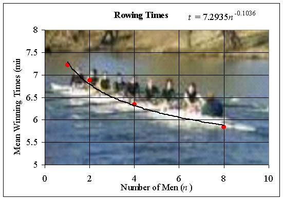
We see that the best fitting power law agrees well with our model from dimensional analysis.

Dimensional analysis

In the above problem we simply used similarity arguments and used proportionalities to obtain estimates for winning times of racing shells. The use of dimensions can prove very useful as a check on the algebra of your problem also. For example, if the left hand side of the equation has units concentration per time [ML³/T], then so must any of the quantities on the right side of the equation. We shall examine this idea again in our compartmental models. Let us find the dimensions of the spring constant in Hooke's law which says that the force of a spring is proportional to the distance the spring is stretched,

F = kx or k = F /x.

The units of force are [ML/T ²], and for distance the units are [L] which makes the units for the spring constant [M/T ²].

Let us use this analysis to analyze the power in a wind mill. Suppose the wind blows with velocity V [L/T] at a windmill whose area facing the direction of the wind is A [L²]. The only relevant physical constant we need is r [M/L³] , the density of air. The dimension of power P (energy per unit time) is [ML²/T ³]. If we say that the power is proportional to some product of V, A, and r or ..

P = kV ^aA^br ^c,

then it's not hard to see that c = 1, a = 3, and b = 1 or

P = kV ³Ar.

We can use this information to determine what effect on power have by changing the different parameters in our system. . output we will

References:

[1] T. A. McMahon (1971). "Rowing: A similarity analysis," Science 173: 349-351.

[2] E. K. Yeargers, R. W. Shonkwiler, and J. V. Herod, 1996, An Introduction to the Mathematics of Biology: with Computer Algebra Models, Birkhäser, Boston.