![]()
Math 636 - Mathematical Modeling
Fall Semester, 2007
Discrete Modeling - U. S. Population
San Diego State University -- This page last updated 30-Aug-07
|
|
Math 636 - Mathematical Modeling |
|
|---|---|---|
|
San Diego State University -- This page last updated 30-Aug-07 |
![]()
Discrete Modeling - U. S. Population
Outline of Chapter
This section compares and contrasts three discrete models for simulating the population of the U. S. We develop the simplest Malthusian growth model, then extend this model in two directions to show a nonautonomous Malthusian growth model and the classic logistic growth model. These models are all fit to census data using a nonlinear least squares best fit. Procedures using Excel and MatLab are presented for finding the best fits and projections are given for each of the models.
Population of the United States
The United States takes a census of its population every 10 years. The census has important ramifications for many aspects of our society, such as budgeting federal payments and representation in Congress. The method of taking the census and how it is analyzed has been a very hot issue pitting the Republicans against the Democrats in 1999 with the issue landing in the Supreme Court. The Republicans wanted a strict interpretation of the Constitution, knowing that a direct head count always undercounts minorities and the poor, who vote predominantly Democratic. The Democrats claimed that the Constitution framers wanted an accurate count of the populace, so that modern statistical methods should be employed. This would naturally give them an advantage in the voting. (The Supreme Court came down in the middle pleasing neither party and saying that the Constitution requires a head count, which will be used for allocating Congressional seats and districting, while the more accurate statistical count may be used for apportioning the money for Federal funding.) The arguing over the numbers will go on for several years as each group tries to use the numbers to their best advantage to gain federal money and political power. Despite the political controversy over the numbers, accurately predicting these demographic data are important for planning our communities in the future. At the base of all calculations for the future population predictions is some type of mathematical model. Current models are quite sophisticated, but first we must appreciate the basic models behind them. Below we present the census data for the history of the U. S.
|
U. S. Census Data |
|||||
|---|---|---|---|---|---|
|
|
3,929,214 |
|
39,818,449 |
|
151,325,798 |
|
|
5,308,483 |
|
50,155,783 |
|
179,323,175 |
|
|
7,239,881 |
|
62,947,714 |
|
203,302,031 |
|
|
9,638,453 |
|
75,994,575 |
|
226,545,805 |
|
|
12,866,020 |
|
91,972,266 |
|
248,709,873 |
|
|
17,069,453 |
|
105,710,620 |
|
|
|
|
23,191,876 |
|
122,775,046 |
||
|
|
31,433,321 |
|
131,669,275 |
||
The growth rate between each decade can be determined by dividing the census at one date by the census a decade earlier and subtracting one. The growth rate for the decade of 1790-1800 35.1%. The javascript below performs this computation to give the growth rate for any decade in the history of the U. S.
From the javascript above, we find that the growth rates for decades following 1790, 1800, and 1810 are 35.1%, 36.4%, and 33.1%, respectively, which averages 34.9% per decade. This growth rate remains almost constant until 1860, so this information should allow us to estimate the census data up until 1860 using a model with a constant growth.
The simplest mathematical model is the Malthusian growth model, which states that
where r is the average growth rate. Thus, the population in the next decade is equal to the current population plus the current population times the average growth rate, r, of the population. This equation is the Discrete Malthusian Growth model (named after the work of Thomas Malthus (1766-1834)). If we begin the model at the population in 1790 and use the average growth rate, r = 0.349, from above, then the table below shows the predictions by this model through 1870 along with the percent error from this model.
|
|
|
|
|
|
|
|
|
|
|
|
|
|
|
|
|
|
|
|
|
|
|
|
|
|
|
|
|
|
|
|
|
|
|
|
|
|
|
|
|
|
|
|
|
|
|
|
|
|
Notice that the error remains small until 1870 because of the fairly constant rate of growth. Most of the predicted populations are a little high, especially in 1870, suggesting that throughout the 19th century the growth rate declined. The declining growth rate is a general trend that we observe for the U. S. and is something that needs to be accounted for in any improved model. Between 1860 and 1870, the Civil War occurred, which is one cause of the dramatic decline in the rate of growth of the population in the U. S. Thus, the 1870 prediction is one that you would expect to be poor. In fact, the shift from the primarily agricultural society to the industrial revolution is more significant in causing the decline in the rate of growth. The crowding effects are what the logistic growth model considers.
Clearly, the Malthusian growth model is limited to a range of dates where the growth rate remains relatively constant. If you attempt to continue using this model until 1920 or 1970, then the model produces the census values of 192,365,343 and 859,382,645, respectively. (These estimates are 82% and 323% too high.) Thus, this model becomes increasingly bad if we assume the constant growth rate of 34.9%. A calculation of the growth rate in 1920 gives around 15%, which further drops to only 13% in 1970. (The lowest growth rate can be seen to have occurred during the Great Depression (between 1930 and 1940) with only a 7.2% growth rate.) Thus, this simple model can only predict populations for a limited time into the future, but certainly provides good estimates for some community planning that is required.
Solution of Discrete Malthusian Growth Model
There are not many discrete models that have an explicit solution. However, it is easy to solve the discrete Malthusian growth model. From the model above, we see that
P2 = (1 + r)P1 = (1 + r)2P0, ...
Pn = (1 + r)Pn-1 = ... = (1 + r)nP0.
Thus, the general solution of this model is given by
This shows why Malthusian growth is also known as exponential growth. The solution to the model that is given by the equation above is an exponential function with a base of 1+ r and power n representing the number of iterations after the initial population is given.
Improving the Malthusian Growth Model
The section above presents a discrete Malthusian Growth model based on the U. S. population from census data. From the solution to the model above, we see that the Malthusian growth model has only two parameters that can be adjusted, the initial condition, P0, and the growth rate, r. In this section, we examine two extensions of the Malthusian growth model that increase the number of modeling parameters to three. One model extends the Malthusian Growth model to include time varying reproduction rates, and the other model is the classical logistic growth model. We will compute the least squares best fit of all models in this section to see how they do at matching the census data and discuss the model predictions for the future. A hyperlink is provided to the Excel worksheet with the U. S. population models, and below we present MatLab computations for finding the least squares best fit to the logistic model.
The general discrete dynamical population model is given by
where f is a function depending only on the population P at time tn. This difference equation is said to be autonomous as it does not have a temporal or time dependence. A more general difference equation is given by
which is a nonautonomous difference equation.
As noted above, the general solution of the Malthusian growth model is given by
A nonlinear least squares best fit to the census data gives the best fitting parameters to this model as the initial condition, P0 = 15.07, and the growth rate, r = 0.1524. Thus, the best fitting model is given by
Pn = 15.07(1.1524)n.
This model poorly fits the early and late census data, but it is extremely simple with only two parameters. The sum of square errors is 2297.
We know that human populations vary with technology and medical care much more than other animal populations. This suggests that a time varying growth rate would provide a better model. It is clear from the census data that the growth rate over the last two centuries has been declining. A linear growth rate in time adds only one parameter, but proves to create a substantially better fit to the census data. The nonautonomous Malthusian growth model with linear time varying growth is given by
where a and b are parameters to be fitted to the data and tn = 10n is the time after 1790 in years. We now have three parameters: the initial condition, P0, and the growth parameters, a, and b. A nonlinear least squares best fit to the census data gives the best fitting parameters to this model as the initial condition, P0 = 5.877 , and the growth parameters, a = -0.001062 and b= 0.3092. Thus, the best fitting model is given by
Pn+1 = (1.3092 - 0.01062 n )Pn,
with P0 = 5.877. This model fits the census data quite well, and the sum of square errors is only 300.1.
The earliest and most famous of the autonomous models that extend beyond Malthusian growth is the logistic growth model. This model has been shown to fit many animals populations with limited resources quite well. So we can ask how well the human population follows this model. The logistic growth model also has three parameter. The logistic growth model is given by
where r and M are parameters to be fitted to the data with the initial condition, P0. A nonlinear least squares best fit to the census data gives the best fitting parameters to this model as the initial condition, P0 = 7.992 , and the growth parameter, r = 0.2342 and carrying capacity, M= 408.4 . Thus, the best fitting model is given by
Pn+1 = (1 + 0.2342(1 - Pn/408.4 )Pn,
with P0 = 7.992. This model fits the census data quite well, and the sum of square errors is only 491.9. The sum of square errors shows that the logistic growth model is only a slightly poorer fit to the data than the nonautonomous Malthusian growth model.
The graph below gives a comparative study of these three models. The Malthusian Growth model performs poorly as noted above because the growth rate varies too much over the time interval being considered. The Nonautonomous Discrete Malthusian Growth and Logistic Growth models match the data quite well.
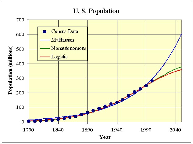
The analyses above and the graph above were computed using Excel's nonlinear Solver routine, which is a complex algorithm for finding minima (or maxima) of functions by varying parameters. The complete worksheet is available for downloading. Similar calculations can be easily done with MatLab using its fminsearch routine.
The simulations of the models given above into the future project that the population in 2050 and 2100 are 602.3 and 1,224 million according to the Malthusian growth model, 378.4 and 401.2 million according to the nonautonomous Malthusian growth model, and 358.7 and 393.6 million according to the logistic growth model. The nonautonomous growth model predicts that the maximum population in the U. S. will occur between 2080 and 2090 with the maximum being about 405 million. The logistic growth model predicts that the population will increase less and less rapidly, leveling off around 408 million. It is rather remarkable how similar the predictions of the nonautonomous Malthusian and logistic growth models are.
Nonlinear Least Squares Fit with MatLab
It is not difficult to create a matlab program to find the least squares best fit to the U. S. census data. Begin by loading the U. S. Population data. In MatLab, we write
usdata = load('USpop.dat);
We create function for simulating the logistic growth model.
function pop=dislog(p)
pop(1) = p(1);
for n = 1:20
pop(n+1) = pop(n)+p(2)*pop(n)*(1-pop(n)/p(3));
end
This function depends on the three parameters given above, and they are stored in the vector p with P0 = p(1), r = p(2) and M = p(3). A function is created to compute the sum of square errors
function err=lstsquares(p)
usdata=load('USpop.dat');
pop = dislog(p);
e1 = usdata(:,2)'-pop;
err = e1*e1';
Next we use fminsearch to compute the least sum of square errors and store the information in the variable p1 as follows:
p1 = fminsearch(@lstsquares, [3.9, 0.25, 400])
If we type the following, then we obtain a nice plot of the data and model:
pop = dislog(p1);
t = usdata(:,1);
plot(usdata(:,1),usdata(:,2),'o',t,pop,'-')
Equilibria
This section extends our study of discrete dynamical equations to nonlinear functions in order to find what can be learned about their qualitative behavior. The linear discrete dynamical models were introduced before the sections on differentiation showing the modeling of populations with Malthusian growth and other linear models, such as one for breathing. As noted above, there is no general solution for the logistic growth model. However, we would like to learn more about this very important model from population biology. Here we introduce the key steps for studying the qualitative behavior of discrete dynamical equations.
Consider the general discrete dynamical equation:
Pn+1 = f(Pn).
The first step in any analysis of a discrete dynamical equation is finding equilibria, which is simply solving an algebraic equation. An equilibrium point of a discrete dynamical system is a point where there is no change in the variable from one iteration to the next. Mathematically, this occurs whenever there is a solution to
Pe = f(Pe).
Graphically, this is when f(Pn) crosses the line Pn+1 = Pn, the identity map, which is one reason why this line was shown above.
Consider the original discrete Logistic equation listed above with r > 0. The equilibria are found by solving:
Thus, the equilibria for the Logistic growth model are either the trivial solution 0 (no population) or the carrying capacity M.
Watch what happens in the applet above as we choose different values of r. For example, try the values r = 0.5, 1.8, 2.3, and 2.65. (Note that the solution of the discrete Logistic equation only gives solutions at the integer values of n, so the connecting lines are only drawn to help visualize the behavior of the system.) The first value of r shows the curve smoothly ascending to carrying capacity of 1000. The second value of r has the population ascend and actually overshoot 1000, then oscillates about 1000, getting closer to the carrying capacity as n increases. In both of these cases, the equilibrium population of 1000 is said to be stable. When r = 2.3, the solution oscillates about 1000, taking on the values of approximately 690 and 1180. This solution is said to have a period of 2. The last case shows the population oscillating almost randomly about 1000. This last situation could have either a very high period of oscillation or actually be chaotic. See what happens when you change the value of M.
Stability of the Logistic Growth Model
Robert May (1974) demonstrated that the discrete Logistic growth model could display very complicated dynamics. As the parameter r increases (assuming that r > 0), then the discrete logistic growth model has the equilibrium at M begin as being monotonically stable with solutions smoothly approaching this equilibrium. After r > 1, the solution oscillates and approaches the equilibrium at M. Further increases in r results in first a period 2 behavior (solutions approaching two distinct values), then a series of period doublings until the system goes into chaos. This behavior can be studied in more detail in the dynamical systems courses offered here.
We would like to have some mathematical tools that help us predict some of these behaviors. If we write the discrete logistic growth model
then the derivative of the function f(P) proves to be a valuable tool for determining the behavior of the discrete dynamical system near an equilibrium point.
The discrete logistic growth model, as given by the equation above, has two equilibria,
Pe = 0 and Pe = M.
It is easy to see that the derivative of f(P) is given by
f '(P) = 1 + r - 2 rP/M.
At Pe = 0, the derivative satisfies
f '(0) = 1 + r,
which for r positive always results in solutions growing away from this equilibrium. (If r is a negative number between -1 and 0, then the solution of the discrete logistic growth model decays to 0 or the population goes to extinction.)
The more interesting behavior occurs around the second equilibrium, Pe = M. Below is a summary of the types of behavior that are observed for a discrete dynamical system near an equilibrium, Pe. (In all of the descriptions below, we are assuming that the simulation begins "near" the equilibrium value.)
Behavior of the Discrete Dynamical Model near an Equilibrium
Returning to the logistic growth model, we can evaluate the derivative at the larger equilibrium, Pe = M. From the formula for the derivative, it is easy to see that
f '(M) = 1 - r.
From our list of behaviors above, it is follows that
[1] Statistical Abstracts of the United States (1993) 113 th ed., U. S. Department of Commerce, Bureau of the Census, Washington, DC.