Math 536 - Mathematical Modeling Fall Semester, 2000
	© 1999, All Rights Reserved, SDSU & Joseph M. Mahaffy San Diego State University -- This page last updated 11-Jan-00

The best known technique for fitting data to a given function is the method of least squares. This technique assumes that the x values of the data are correct, then the difference between the y values of the data and the y values of the proposed model function are evaluated at each x value in the data set. The sum of the squares of these errors is then minimized with respect to the parameters in the model function. For a straight line, the parameters that can be adjusted are just like the sliders on the applets that you played with in the main section, the slope of the line and the intercept. (Note that the model function need not be a straight line to apply this technique, but our analysis below will only examine the case of a straight line model.)

In this section we examine how to find the best fit to a straight line. We are given a data set consisting of n data points: (x₁, y₁), (x₂, y₂), ... , (x_n, y_n). The mathematical model is a straight line given by the formula

We need to select a slope, a, and an intercept, b, that minimizes the square of the error in the distance between the y_i values of the data points and the y value of the line. As noted in the main section, the error between each of the data points and the line are given by

The least squares best fit is found by minimizing the function

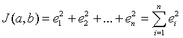
with respect to the variables a and b. (This is done by taking the partial derivatives of J(a,b) with respect to a and b and setting these partial derivatives equal to zero. In this course we will be learning about derivatives and how they relate to finding minimum values of functions.) Note that the symbol S is summation notation and is used to shorten the amount of writing we need to use. It simply stands for adding together a collection of similar terms.

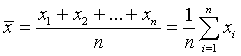
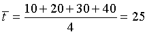
The details of this analysis are omitted, since it does require a little more knowledge of Calculus. However, the results are summarized below. First, to make the calculations more manageable, we define the mean of the x values of the data points as

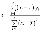
The value for the slope of the line that best fits the data is given by

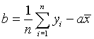
With the slope computed, the intercept is found from the formula

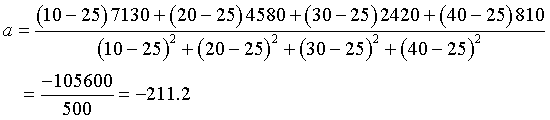
Example: Let us apply this to our example beginning the main section. There are four data points in the E. coli example, (10,7130), (20,4580), (30,2420), and (40,810). First we compute the mean of the times

The slope a is found by the following calculation.

Similarly, the c-intercept, b, is readily computed to give

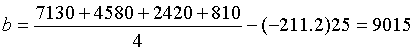
The answer on the main page rounds the values of a and b to three significant figures.