Math 536 - Mathematical Modeling Fall Semester, 2000
	© 1999, All Rights Reserved, SDSU & Joseph M. Mahaffy San Diego State University -- This page last updated 29 August-00

1. Cumulative AIDS cases
2. Allometric or Power Law Model
3. Finding Allometric Models
4. Log-Log Graphs
5. References
6. Problems

Cumulative AIDS cases

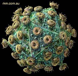
The advent of AIDS in modern society has had a significant impact on both personal behavior and public policy. The new protease inhibitors have significantly improved the quality of life for those who are HIV positive; however, this has come at a substantial cost to society. The new drugs are extremely expensive, are difficult to take because of the complex scheduling requirements to be effective, and have many strong side effects (besides not always working for a particular person or strain of the HIV virus). In turn, there are a number of people who are now avoiding safe sex practices as they no longer fear the "Death Sentence" that used to be associated with an HIV infection. Below is a figure illustrating the HIV virus. It has links to more images with more details about the virus.

 

	......
..		..
	[click for enlarged and detailed image] illustration by Russell Kightley Media, all rights reserved http://www.rkm.com.au

There is an important need for our society to know the extent of this disease from both an economic and sociological perspective. In order to make informed public policy, we need to know what is the expected case load in the upcoming years. However, it is clearly an extremely complex modeling problem. Below is a table of cumulative cases of AIDS between 1981 and 1992 [1] and an animated .gif showing the spread of the disease (through mortality statistics) over a similar period of time..

..		..
	click here to view mpeg

A quick glance at the data will clearly show that it is not linear, so a linear model is not appropriate. However, these techniques are very complicated an often difficult to implement. A hyperlink provides an applet for finding the best nonlinear least squares fit to the data for cumulative AIDS cases, which is different from the technique we'll show below

Allometric or Power Law Model

As noted above, using a least squares fit to nonlinear data can be extremely difficult. However, there are a few standard nonlinear models used in biological applications that are more easily analyzed. The technique that we'll develop in this section is known as the Power Law of Modeling. It is also referred to as Allometric Modeling. Allometric models are used regularly in modeling complex biological phenomena where the actual mechanisms underlying the model behavior are too complex to describe in detail, but there is a need to be able to make some predictions.

Allometric models assume a relationship between two sets of data, x and y, that satisfy a power law of the form

where A and r are parameters that are chosen to best fit the data in some sense. Note that this model assumes that when x = 0, then y = 0. As always, you should be aware of the limitations of this type of modeling. This method provides its best predictive capabilities when examining a situation that lies between the given data points. For example, if the number of species of herptofauna on Carribean islands is determined for a collection of islands with varying areas, then this model would give a reasonable estimate for the expected number of species on another Carribean island with an area that lies between the collected data. It would not be appropriate for extending to a large continent as the area is significantly beyond the range of the collected data. It wouldn't even be appropriate for another island such as Iceland, which lies in a different type of climate and has a different geography.

Allometric models are found by taking the logarithms of the data (or graphing the data on log-log graphs) and seeing if the data lie roughly on a straight line. If this is the case, then a power law relationship makes a reasonable model. Below is an applet showing the linear least squares fit to the logarithms of the data for cumulative aids cases, and the graph to the right shows the modeling relationship with a normal scale. The allometric model has x be time in years since 1980 and y be the cumulative AIDS cases.

The applet above can be adjusted until you reach a minimum least squares for the log of the data with J(A,r) = 0.10. The best slope is r = 3.27 and the best intercept is ln(A) = 4.42. We will show later that this gives the best fit power law for this model as

The graph shows that the power law provides a reasonable fit to the data. Unfortunately, the fit is weakest at the end where we'd like to use the model to predict the cumulative AIDS cases for the next year. The model predicts 366,990 cases in 1993, which is clearly too high from the given data. However, the analysis does give some indication of the rate of growth for this disease, which provides a first approximation for improved models and could be applied to expected spread of another disease with similar infectivity as HIV. This modeling technique is still valuable for analysis of many other data sets and occasionally can provide insight into the underlying biology of the problem. A better fit to the data is shown in the nonlinear least squares appendix that can be viewed through the hyperlink. We will see more examples of this in the computer labs.

Below we will show the method for determining the parameters A and r in the model. First, we need to review the properties of exponents and logarithms.

Review of Exponents and Logarithms

There are several properties of exponents that you should remember from algebra.

These properties can be used to simplify expressions involving exponents.

To solve equations that have exponents in them, we need to have the inverse function of the exponent. This is the logarithm. If you are given the equation,

then the inverse equation that solves for x is given by

The a in the above expression is called the base of the logarithm. Again there are a collection of properties of logarithms that prove useful for solving equations and simplifying expressions.

Note that in the properties of logarithms, we only needed to specify the base of the logarithm for Property 5. All other properties are independent of which base is used. The two most common logarithms that are used are log₁₀ and log_e. The latter logarithm is called the natural logarithm, often denoted log or ln, and is the one most commonly used (and is the default on your calculator). Later you will learn about the importance of the natural base e. For most of our work, we will use the natural logarithm.(Note that Excel defaults to log₁₀.)

Graphing Exponentials and Logarithms

As noted above, the exponential function, e^x, and the natural logarithm, ln(x), are inverse functions of each other. In this section we show the graphs of these functions to develop some sense of their behavior. We will study e^x in greater detail after learning more about the derivative. However, for graphing purposes you need to know that e is an irrational number between 2 and 3, more precisely, e = 2.71828.... The domain of e^x is all of x with becoming extremely small very fast for x < 0 (a horizontal asymptote of y = 0) and growing very fast for x > 0. Its range is y > 0. Similarly, the graph of y = e^-x has the same y-intercept of 1, but its the mirror reflection through the y-axis of y = e^x. It becomes very large for and very small for . A graph of both y = e^x and y = e^-x is given below.

Since ln(x) is the inverse function of e^x, an easy way to graph this function is to mirror the graph of e^x through the line y = x. The domain of ln(x) is x > 0, while its range is all values of y. As y = ln(x) becomes undefined at x = 0, there is a vertical asymptote at x = 0. The graph of y = ln(x) is given below.

We will see that the exponential function plays a role in many applications, so it is very important to understand this function and how its graph behaves. Several examples are illustrated in the hyperlinked  Worked Examples for Exponentials and Logarithms section.

Finding Allometric Models

We return to the Allometric model developed above, where two sets of data, x and y are assumed to satisfy a power law of the form

We want to choose the parameters A and r that best fit the data. The next step is to take the logarithm of both sides, then use the properties of logarithms to simplify the equation.

From this formula, we see that if we take the logarithm of the data, ln(x) and ln(y) and graph it we should see a straight line. That is, if we take X = ln(x), Y = ln(y), and a = ln(A), then the above equation can be written Y = a + rX , which is a line with a slope of r and a Y-intercept of ln(A).

We return to the example at the beginning of this section. Below is a table that includes both the data and the logarithms of the data.

Below shows a graph of the logs of the data (year-1980 and cumulative AIDS cases) along with the best straight line fit.

The plot above shows that when the logarithms of the data for the cumulative AIDS cases are plotted against the logarithms of the time since 1980, then these logarithmic data lie fairly close to a straight line. The least squares best fit of the straight line to the logarithms of the data give a slope of r = 3.274 and intercept of a = ln(A) = 4.415, which gives A = 82.70. Whenever this is the case, then an allometric or power law model makes a reasonable description of the data.

Log-Log Graphs

There exist graphing routines that readily create what is known as a log-log plot. This allows the user to simply graph the data directly onto a graph with logarithmic scales on the axes to see if the data falls on a straight line suggesting an allometric or power law model. Below we show a plot of the original data on cumulative AIDS cases against the date - 1980 on a graph with logarithmic scaled axes.

Example: Consider the relationship between weight and pulse. We know that smaller animals have a higher pulse than larger animals. Let us assume that this relationship satisfies an allometric model. Later in Lab we will perform a more detailed study of this phenomenon to check on the validity of using the allometric model (or power law).

We are given that a 17 g (or .017 kg) mouse has a pulse of 500 beats/min. Assume a 68 kg human has a pulse of 65. Let us use these data to form an allometric model and predict the pulse for a 1.34 kg rabbit. The power law gives

Next we take logarithms to obtain:

As noted above, this is a straight line in ln(P) and ln(w) with slope of k and intercept of ln(A). From the data,

The slope k is given by:

We can use this slope with one of the points to find ln(A) as follows:

Thus,

If we use the first equation with a 1.34 kg rabbit, then it gives P = 171.

Kepler's Third Law

This example relates to Kepler's Third Law. We will use the power law to determine the period of revolution about or distance from the sun for all planets given information about some of the planets. Let d be the mean distance (x10 ⁶ km) from the sun and p be the period of revolution in days about the sun. Here are data on four of the planets:

The power law expression relating the period of revolution (p) to the distance from the sun (d) is given by

where k and a are constants to be determined. We use the power law under Excel's trendline to best fit the data above. The graph below gives the best power law fit, showing k = 0.1995 and a = 1.5002. The power law clearly fits the data very well.

We saw that a straight line fits the logarithms of data that satisfy the power law, giving ln(p) = ln(k) + a ln(d) from the formula above. In the table above, take the logarithm of the Distance (ln(d)) and the logarithm of the Period (ln(p)). Here we'll use Excel's scatter plot and linear fit under trendline to see how this fits the data. The coefficient a agrees with the power a above, and exp(-1.6122) = 0.1994, which is almost the coefficient k found above. Again this straight line agrees extremely well with the data.

So now we use this power law to test the model against the other planets. Below is a table showing the calculated distance or period given either the distance or period of the planet along with the error from data taken from the Jet Propulsion Laboratory website

(The bold numbers are the calculated numbers, while the other number is the one given.)

References:

[1] E. K. Yeargers, R. W. Shonkwiler, and J. V. Herod, 1996, An Introduction to the Mathematics of Biology: with Computer Algebra Models, Birkhäser, Boston.

Problems:

1. Research has shown that the average number of mammalian species N on an island satisfies the equation

N = kA^1/3

where A is the area (in km²) of the island and k = 2.

a.Find the expected number of mammals on islands with 125 and 8000 km².

b. If you discovered an island had 32 different species of mammals, then, based on the formula above, approximately how large is the island?

c. Sketch a graph of the number of mammalian species on an island vs. the area of the island. Plot the points found in Parts a and b.

2. The Crew Classic rowing event on Mission Bay is held each year in spring. It can be shown that the times, t, of a particular race satisfy a power law with respect to the number of men, n, in the boat,

i.e. t = kn^a

You are given that the winning time for the eight man crew was exactly 6 min., while the winning time for the four man crew was 6min 28.8 sec (Remember to convert the seconds to decimal minutes.)

a.With the information given above find the value for k and a.

b. Use your answer from part a to determine likely winning times for the pairs (2 oarsmen) and singles (1 oarsman).

3. Data suggest that the lifetime of erythrocytes (red blood cells) for mammals satisfy an allometric model. The average lifetime for erythrocytes in a 70 kg man is 120 days. The average lifetime for erythrocytes in a 1.5 kg rabbit is 65 days. Use these data to find an allometric model for the lifetime of erythrocytes as a function of weight, i.e.,

Find the constants k and a. Use this model to determine the average lifetime for erythrocytes in a 20 kg dog. Also, determine the weight of an animal whose erythrocytes live for 100 days.

 4. In Gulliver's Travels, the Lilliputians decided to feed Gulliver 1728 times as much food as a Lilliputian ate. They reasoned that, since Gulliver was 12 times their height, his volume was 12³ = 1728 times the volume of a Lilliputian and so he required 1728 times the amount of food one of them ate. Why was their reasoning wrong? What is the correct answer?

5. Currently there is a debate on the importance of preserving large tracts of land to maintain biodiversity. Many of the arguments for setting aside large tracts are based on studies of biodiversity on islands. In this problem you apply the power rule to determine the number of species of herpetofauna (amphibians and reptiles) as a function of island area for the given Caribbean islands. You are given the following data [1]:  

Island	Area (mi 2)	Species
Redunda	1	3
Montserrat	33	10
Jamaica	4,411	38
Cuba	46,736	97

 a. Let N be the number of species and A be the area of the island, then the power law expression relating the number of species to the area of the island is given by

Use the power law under Excel's trendline to best fit the data above. Plot the data and the best power law fit, then have Excel write the formula on your graph. How well does the graph match the data?b. For allometric models, we have seen that we could fit a straight line to the logarithms of data that satisfy the power law, giving

In the table above, take the logarithm of the Number of Species (ln(N)) and the logarithm of the Island Area (ln(A)). Use Excel's scatter plot and linear fit under trendline to see how this fits the data. Plot a graph of the logarithm of the data and the best straight line fit to these data. Show the formula for this straight line on your graph. Compare the coefficients obtained in this manner to the ones found in Part a. How well does the graph match the data?c. From your calculations above give estimates to fill in the table below.  

Island	Area (mi 2)	Species
Saba	5
Puerto Rico		40
Saint Croix	80
Hispaniola		88

 d. How important is maintaining a large tract of land to the maintenance of biodiversity based on this model? What does the model predict is required in increased preserved area to double the number of species supported by the environment? Write a short paragraph explaining your results as best you can.

[1]Data from J. Mazumdar, An Introduction to Mathematical Physiology and Biology , Cambridge, 1989.