|
|
Math 122 - Calculus for Biology II |
|
|---|---|---|
|
San Diego State University -- This page last updated 31-Mar-04 |
Riemann Sums and Numerical Integration - Examples
|
|
Math 122 - Calculus for Biology II |
|
|---|---|---|
|
San Diego State University -- This page last updated 31-Mar-04 |
This section works a number of examples using the numerical integration techiques.
Example 1: Find the area in the first quadrant under the curve
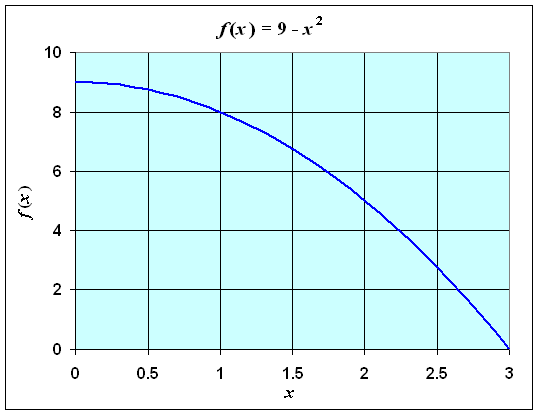
f(x) = 9 - x2.
Sketch a graph showing the area under the graph, then use the Midpoint rule and the Trapezoid rule to approximate the integral with n = 3 and n = 6. Since this is a quadratic, use Simpson's rule to give the exact answer with n = 6.
Solution: The graph below shows the region of interest.

It follows that we are interested in approximating the definite integral given by

For n = 3, the three subintervals are [0,1], [1,2], and [2,3], and the value of Dx is 1.
For the Midpoint rule, the midpoints are c1 = 0.5, so f(1/2) = 8.75, and c2 = 1.5, so f(1.5) = 6.75, and c3 = 2.5, so f(2.5) = 2.75. The Midpoint rule gives

For the Trapezoid rule, the integral approximation formula gives

For n = 6, thesix subintervals are [0, 0.5], [0.5, 1], [1, 1.5], [1.5, 2], [2, 2.5], and [2.5, 3], and the value of Dx is 0.5.
For the Midpoint rule, the midpoints are c1 = 0.25, so f(0.25) = 8.9375, c2 = 0.75, so f(0.75) = 8.4375, c3 = 1.25, so f(1.25) = 7.4375, c4 = 1.75, so f(1.75) = 5.9375, c5 = 2.25, so f(2.25) = 3.9375, and c6 = 2.75, so f(2.75) = 1.4375. The Midpoint rule gives

For the Trapezoid rule, the integral approximation formula gives

In each of the cases above, we see that the midpoint rule is over estimating the integral and the trapezoid rule is under estimating the value.
The actual value of the integral is found using Simpson's rule. Simpson's rule requires that n be even, so with n = 6 we have Simpson's rule for this quadratic function giving the exact value:

Thus, the area under this quadratic expression in the first quadrant is 18. The calculations above show that the midpoint rule and trapezoid rule give fairly good approximations, so these numerical techniques provide a valuable method of approximating integrals, but Simpson's rule requires little extra work and gives significantly better results. The next section will show how to use the fundamental theorem of Calculus to obtain this area directly from integration techniques.
Example 2: Insects are an important agricultural pest, and some pesticides have there greatest effects at particular stages of the insect development. Timing of application of the pesticide can be very significant. However, the maturation of insects is often dependent upon temperature more than length of time. Thus, it can be important to track the cumulative temperature rather than the length of time that an insect has been around. Cumulative temperature Tc (in oC-hr) is found by integrating the temperature T(t) over a period of time.

Suppose that the following data are found on the temperatures for part of a day (between Noon and 7 PM).
|
Time |
12:00
|
13:00
|
14:00
|
15:00
|
16:00
|
17:00
|
18:00
|
19:00 |
|
Temp (oC) |
33
|
34
|
36
|
35
|
32
|
30
|
26
|
24
|
Use the Trapezoid rule and the data from the table to approximate the cumulative temperature from noon to 7 PM.
Solution: Since the length of time between the temperature measurements is one hour, Dt = 1. The trapezoid rule for approximating the integral gives

Note that this varies only slightly from computing the average temperature and multiplying by the length of time.