1. Competition Model for Yeast
2. Euler's Method for a System of Differential Equations
3.  
4. References

This section extends our work on two dimensional differential equations to numerical methods and some graphical techniques for understanding their behavior. The section begins by showing numerical methods for solving the systems of differential equations developed in the sections on the Lotka-Volterra predator-prey system and the model for competition of two species of yeast. These numerical solutions allow finding the best parameters that fit the data of the mathematical model (though these nonlinear least squares fitting techniques are beyond the scope of this course, so are simply outlined using Excel's solver routine).

Competition Model for Yeast

In the previous section, a mathematical model for the competition of two species of yeast was presented along with an equilibrium analysis. The mathematical model for competition of two species was given by the following system of differential equations

In that section, the data for the Gause experiments on the two yeast species S. cerevisiae and S. kephir were presented. The parameters a₁, a₂, b₁, and b₂ were computed by using a nonlinear least squares fit to the data for the experiments where the species were grown in pure cultures. The parameters a₁ and b₁ represent the growth rate of the species S. cerevisiae and S. kephir, respectively, while the parameters a₂ and b₂ represent the intraspecies competition of S. cerevisiae and S. kephir, which can be used to find the carrying capacity of these species growing individually. The question remains on how we can find the remaining parameters a₃ and b₃, which represent the interspecies competition.

The data we want to match is presented again below:

Time (hr)	0	1.5	9	10	18	18	23	25.5	27	38	42	45.5	47
Volume (S. cerevisiae)	0.375	0.92	3.08	3.99	4.69	5.78	6.15	9.91	9.47	10.57	7.27	9.88	8.3
Volume (S. kephir)	0.29	0.37	0.63	0.98	1.47	1.22	1.46	1.11	1.225	1.1	1.71	0.96	1.84

These data are more scattered than the monocultures. If we make an assumption that these cultures first approach a coexistence equilibrium near X_e = 9 and Y_e = 1.8. Recall that the coexistence equilibrium is given by

Since the monoculture studies gave the parameters a₁ = 0.2586, a₂ = 0.02030, b₁ = 0.05744, and b₂ = 0.009768, we can estimate values of a₃ and b₃ from the equations above and estimates of the coexistence equilibrium. The simultaneous solution of these two nonlinear equations (using a program such as Maple's solve routine) give either a₃ = 0.0422 and b₃ = 0.00443 or a₃ = 0.044 and b₃ = 0.00451, which are solutions that are close enough for initial estimates in a nonlinear least squares fit to the simulation of the data in the table above.

Euler's Method for a System of Differential Equations

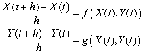
So how do we simulate the data using our competition model? The simplest and most intuitive method for simulating any 2-D system of differential equations is to use Euler's method, which we developed earlier this semester for solving a nonlinear differential equation. The idea behind Euler's method is to use the definition of the derivative

but choose a specific value of h, the stepsize of the iteration scheme, instead of finding the limit as h becomes very small. This results in our differential equations changing from a system of continuous equations involving two unknown functions and their derivatives to a discrete dynamical system of two unknown variables, which are easily simulated using the computer.

Fix the stepsize h, then use the discretized form of our system of differential equations above. The result is the following system of equations:

If we define X(t+h) = X_n+1, X(t) = X_n, Y(t+h) = Y_n+1, Y(t) = Y_n, then after a little algebra, the system of equations above can be written

Thus, by knowing the initial values X₀ and Y₀ and the stepsize h along with the functions f(X_n, Y_n) and g(X_n, Y_n),  then we can easily compute the subsequent values X_n and Y_n for n = 1, 2, 3, ... This gives us a numerical approximation to the solution of the system of differential equations, and this iteration scheme is known as Euler's method for solving a 2-D system of differential equations.

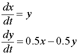
Example 1: Consider the system of differential equations given by

with the initial conditions

Use Euler's method with a stepsize of h = 0.5 to approximate the solution at t = 2.

Solution: From the information above the Euler's iteration scheme with a stepsize of h for this system of differential equations is given by

with the initial values x₀ = 1 and y₀ = 2. We need to perform 4 iterations of this scheme to obtain the approximation at t = 2. The first iteration, which approximates the solution at t = 0.5, is given by

x₁ = x₀ + 0.5y₀ = 1 + 0.5(2) = 2

y₁ = y₀ + 0.5(0.5x₀ - 0.5y₀) = 2 + 0.5(0.5(1) - 0.5(2)) = 1.75

This process is repeated giving the approximate solution at t = 1 as

x₂ = x₁ + 0.5y₁ = 2 + 0.5(1.75) = 2.875

y₂ = y₁ + 0.5(0.5x₁ - 0.5y₁) = 1.75 + 0.5(0.5(2) - 0.5(1.75)) = 1.8125

and the approximate solution at t = 1.5 as

x₃ = x₂ + 0.5y₂ = 2.875 + 0.5(1.8125) = 3.78125

y₃ = y₂ + 0.5(0.5x₂ - 0.5y₂) = 1.8125 + 0.5(0.5(2.875) - 0.5(1.8125)) = 2.078125

and the approximate solution at t = 2 as

x₄ = x₃ + 0.5y₃ = 3.78125 + 0.5(2.078125) = 4.8203

y₄ = y₃ + 0.5(0.5x₃ - 0.5y₃) = 2.0781 + 0.5(0.5(3.7813) - 0.5(2.0781)) = 2.5039

These calculations are tedious by hand but easily performed by a computer. As we saw with the discrete dynamical systems in Math 121, these computations are very easy to set up and evaluate using spreadsheet software, such as Excel. The spreadsheet for this example is available through this hyperlink.

The solution of this system of differential equations is

References

[1]