1. Random Variable
2. Probability Distribution and Distribution Functions
3. Continuous Probability Density and Distribution Functions
4. Expected Value

This section is designed to introduce the basic concepts in Probability theory. Random variables, probability distributions, and density and distribution functions are defined. Some simple examples from biology are used to illustrate the concepts.

Random Variable

A random variable X is a function with the following properties:

1. X is defined on the sample space S of an experiment, and its values are real numbers.
2. For every real number a, the probability, P(X = a), that X assumes the value a in a trial, is well-defined.
3. For every interval I, the probability, P(X I), that X assumes any value in I in a trial, is well-defined.

Example: Game of Craps

Assuming that a pair of dice are fair, then the sum of the numbers on the two dice represent a set of discrete random variables with well-known probabilities. Thus, the random variables in this case are all the integer values from 2 to 12. The probability of rolling one particular number, say a 5, on one fair die is 1/6. The probability of getting a 5 on the first die and a 2 on the second die is the product of the two individual probabilities, so

One wins at craps if you throw the dice so that they total 7 on the first throw. There are exactly 6 ways that two dice can total 7, (1 on the first, 6 on the second; 2 on the first, 5 on the second; 3 on the first, 4 on the second; 4 on the first, 3 on the second; 5 on the first, 2 on the second; and 6 on the first, 1 on the second). It follows that the probability that our random variable formed by the sum of the numbers on the dice is 7 satisfies

Since there are only 36 possible combinations with two dice, it is easy to compute the probably of any possible range of outcomes of throwing the two dice. If we wanted the probability that our random variable was less than or equal to 4, then there is one way to throw a 2, two ways to throw a 3, and three ways to throw a 4. It follows that

Example: Blood Type

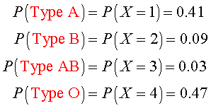
There are 4 primary types of blood, A, B, AB, and O. We can create discrete random variables associated with each of these blood types by assigning integer values to each group. Say we assign 1 to all people with Type A blood, 2 to all people with Type B blood, 3 to all people with Type AB blood, and 4 to all people with Type O blood. From studies of blood types, it has been found that

Probability Distribution and Distribution Functions

Probabilities, which are defined with the random variables, X, from above, form the probability distribution or distribution of X. The distribution function F(x) satisfies

F(x) = P(X < x),

for every x. Note that the distribution function F(x) is always less than or equal to 1.

Examples from Above: Graphs of Discrete Probability Distribution Functions

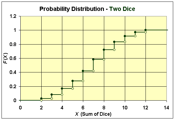
The distribution function for the sum of numbers on two dice is shown below.

The distribution function for the Blood Types is shown below.

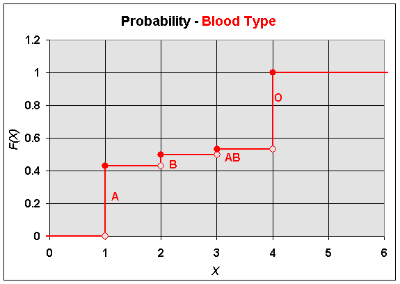
Both of the examples above have discontinuous distribution functions with jump discontinuities equal to the probabilities at each of the integer values.

Continuous Probability Density and Distribution Functions

Many applications have the random variable X varying continuously. We define a density function for a continuous random variable X to be a function with the following properties:

f(x) > 0

The distribution function, F, for the continuous variable X is defined by

Geometrically, the distribution function measures the cumulative area under the density function.

Example: Exponential Decay Density Function

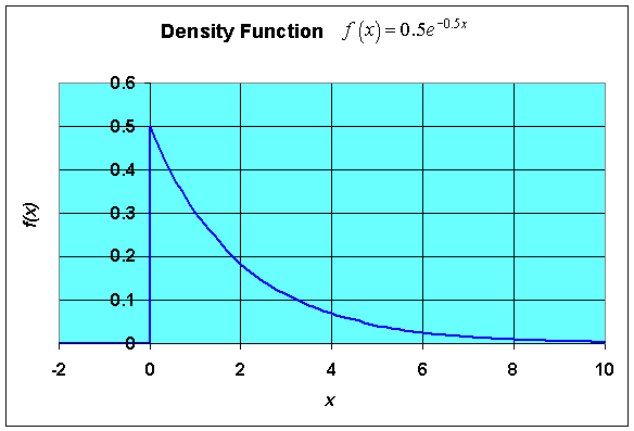
Many biological data can be fit with an exponentially decaying function. This can be seen for seed dispersal of many plants. The continuous density function for a decaying exponential is given by the function

f(x) = ke^-kx, for x > 0.

For x < 0, we assume that f(x) = 0.

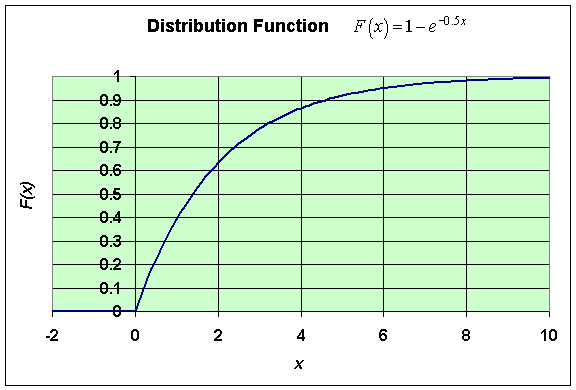
The distribution function, F(x), ( x > 0), for the decaying exponential density function is given by:

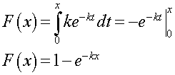
Note that F(x) = 0 for x < 0.

A graph of this density function and distribution function (with k = 0.5) is shown below.

Expected Value of Continuous Density Functions

When the random variable X for some density function f(x) measures some continuous quantity such as the distance, then one can compute the continuous version of the average value of the random variable using the first moment of the density function or the Expected Value of X. This is found by computing the following integral:

We note that the above integral is called an improper integral because of its limits of integration being infinity, which requires additional limiting processes to be considered. This topic is not covered in this course in much detail.

Example: Expected Value for the Exponential Decay Density Function

Consider the exponential decay density function given above, which was defined by

f(x) = ke^-kx, for x > 0.

For x < 0, we assume that f(x) = 0. The expected value for the random variable (or mean of this distribution) satisfies the integral:

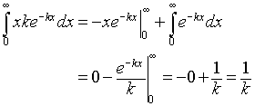
Thus, the expected value or mean for the decaying exponential function, f(x) = ke^-kx is 1/k.