1. Evaluating Definite Inntegrals
2. Area under Curves
3. Average Population
4. Radiation Exposure

This section examines a number of definite integrals. The first part evaluates a couple of definite integrals, then the definite integral is used to find the area under a curve. The section ends with an application to population studies and one on radiation exposure.

Example 1 (Evaluating Definite Integrals):

A. Use the Fundamental Theorem of Calculus to evaluate the integral of f(x) = x³ from -1 to 1.

Solution: The solution is given by

If we want to think of this definite integral in terms of an area, then we see the result no area under the curve. This is because the area under the x-axis is negative, so a function that has odd symmetry over an interval centered on the origin results in the integral being zero.

B. Evaluate

Solution: To integrate this integral we make the following substitution u = 2 - sin(t), so du = -cos(t)dt. The endpoints are t = 0, which changes to u = 2, and t = p/2, which becomes u = 1. Thus, the integral above is solved as follows:

Example 2 (Area under Curves):

A. Suppose we want to find the area under the sine curve from 0 to p. That is we want the area between the curve f(x) = sin(x) and the x-axis. A graph of this region is seen below.

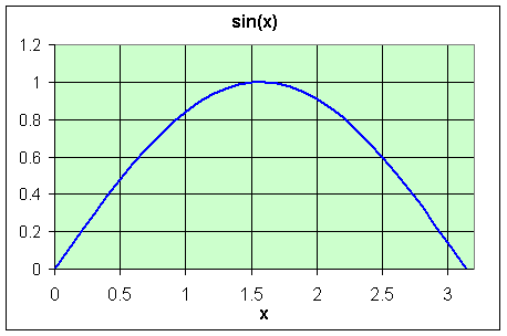
Solution: The area is found by integrating sin(x) on the interval from 0 to p.

B. Find the area between the curves f(x) and g(x), where

A graph of this region is seen below.

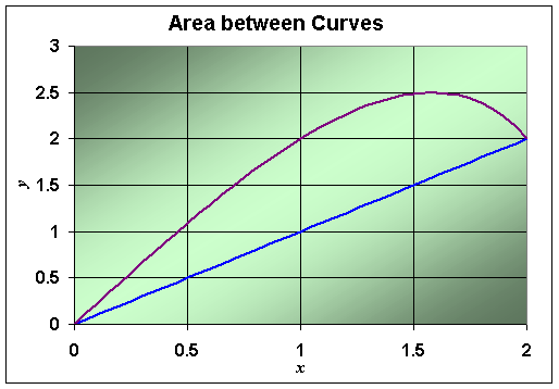
Solution: To find the area between the curves, we must first determine the points of intersection. We solve f(x) = g(x), as follows:

Thus, the points of intersection occur at x = 0 and 2. It follows that the area between the curves is given by the definite integral

The first integral on the right requires the substitution u = 5 - x², so du = -2x dx. The limits of integration change so that when x = 0, then u = 5, and when x = 2, then u = 1. With this substitution, the integral above can be written in the simpler form

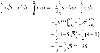
Thus, the area between the two curves is approximately 1.39.

Average Population:

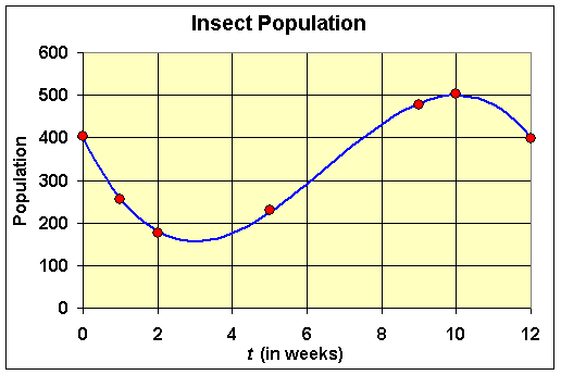
A sample plot of grassland in surveyed for a particular species of insect. Over a 12 week period in the summer, the following data are collected.

A reasonable fit to the data is given by the cubic polynomial

f(t) = 400 - 180t + 39t² - 2t³.

a. Use the polynomial approximation to predict the maximum and minimum populations. Graph the data and the polynomial.

b. Use the data to find the average number of insects in the plot, then use the approximating polynomial to estimate the average number of insects in the plot.

Solution: a. The maximum and minimum populations of these insects are found by differentiating the polynomial. The derivative is given by

f '(t) = -180 + 78t - 6t² = -6(t - 3)(t - 10).

It follows that the relative extrema occur at t = 3 with f(3) = 157 and t = 10 with f(10) = 500. Checking the endpoints, we see that f(0) = 400 and f(12) = 400. Thus, the polynomial predicts that the minimum population occurs at t = 3 with a population of 157, and the maximum population occurs at t = 10 with a population of 500. Below is a graph of the data and f(t).

b. The average of the data given above is easily seen to be 349.1. To find the average population using the polynomial curve, we compute the following definite integral.

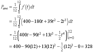
We see that there is a slight difference between the averages, and the better average depends on how you want to interpret your data. In general, the average given by the integral is considered more representative because it gives an even weighting over the time of the experiment.

Radiation Exposure

The integral can be used to calculate the dose from radiation exposure. If the substance has a very long half-life, then the radiation exposure is easily approximated by simply multiplying the amount of radiation measured times the length of time of exposure. However, if the radioactive source is decaying rapidly, then the radiation exposure varies with time.

a. Phosphorous ³²P has a half-life of 14.3 days, undergoing an energetic beta decay (1.7MeV). This radioactive tracer is often used in biological experiments to label nucleotides. Suppose that a hot sample of ATP emits 300 mREM/day. Find the solution to the differential equation

b. The Nuclear Regulatory Commission (NRC) specifies that a laboratory worker can receive 5000 mREM/yr. If the lab worker stays close to this sample, then determine how long the lab worker could remain near the sample before receiving his or her total annual radiation dose.

Solution: a. This differential equation has the solution

R(t) = 300e^-kt.

Because the half-life is 14.3 days, we solve

150 = 300e^-14.3k or e^14.3k = 2.

Thus,

The solution is given by

R(t) = 300e^-0.0485t.

b. The dose that a lab worker receives is based on the rate of exposure times the length of time that the worker is exposed. For rapidly decaying radioactive materials, this is given by an integral of the radioactive decay function integrated over the time of exposure. For our specific example, we have the following integral

where t is the length of time the lab worker is exposed. If the lab worker can receive a body dose of only 5000 mREM/yr, then the allowable dose satisfies the equation

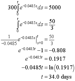
Thus, this lab sample would give the entire annual body dose of radiation to the lab worker in 34 days. Note however, that the lab worker is not likely to be around the sample all the time, and radiation satisfies an inverse square law, so moving some distance away from the sample dramatically lowers exposure. Thus, this sample is unlikely to cause significant exposure even though it is a fairly hot sample.