![]()
Math 121 - Calculus for Biology I
Spring Semester, 2009
Velocity and Tangent Lines
San Diego State University -- This page last updated 14-Mar-09
|
|
Math 121 - Calculus for Biology I |
|
|---|---|---|
|
San Diego State University -- This page last updated 14-Mar-09 |
Differential Calculus began with the study of motion, and Sir Isaac Newton's work on gravity was a key step to the development of Calculus. (There is a controversy as to whether Newton or Leibnitz was the first to invent Calculus.) Gravity plays a key role in biology as well as Physics. This section begins by examining a cat falling from a tree branch. Next the flight of a ball neglecting air resistance is revisited as a classical study in differential Calculus. The flight of a ball and its velocity are used to give a geometric understanding of the derivative by observing how a ball falling under the influence of gravity would appear using a strobe light (and allowed the time of the strobe light to vary).
 The
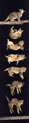
cat has evolved to be one of the best mammalian predators. (Domestic
cats have been shown to responsible for up to 60% of the deaths of
songbirds in some communities.) The domestic cat comes from a line of
cats that adapted to hunting in trees. This requires tremendous
agility. These cats have a very flexible spine that enables them to
spring for prey and absorb the shock from their pouncing. This
flexibility allows them to rotate rapidly during a fall and usually
end up on the ground feet first.
The
cat has evolved to be one of the best mammalian predators. (Domestic
cats have been shown to responsible for up to 60% of the deaths of
songbirds in some communities.) The domestic cat comes from a line of
cats that adapted to hunting in trees. This requires tremendous
agility. These cats have a very flexible spine that enables them to
spring for prey and absorb the shock from their pouncing. This
flexibility allows them to rotate rapidly during a fall and usually
end up on the ground feet first.
Humans have been fascinated by this ability of a cat to right itself so quickly from a fall. There have been quite a few scientific studies of cats falling. One study of cats falling out of New York apartments showed that paradoxically the cats falling from the highest apartments actually fared better than ones falling from an intermediate height. Apparently, the cat first rights itself rapidly during a fall, but remains tense. However, with greater heights the falling cat relaxes and actually spreads its legs to form more of a parachute, which slows its velocity a little and results in a more even impact. From intermediate heights, the cat basically achieves terminal velocity (from the air resistance balancing the force of gravity), but the tension and the stiffness seems to cause increased likelihood of severe or fatal injuries.
The complications of modeling air resistance during a fall are beyond the scope of this course at this time, but we can model the early stages of the fall where the primary dynamics result from acceleration due to gravity. If a cat falls from a tree (not too high up), then its motion is governed by the basic laws of gravity. Newton's law of motion says that mass times acceleration is equal to the sum of all the forces acting on an object. In our introduction to the derivative, we noted that the velocity is the derivative of position. It is also true that acceleration is the derivative of velocity.
Suppose that a cat falls from a branch that is 16 feet high. It can be shown that the height of the cat satisfies the equation
How long does this cat fall and what is its velocity when it hits the ground?
The first question is easily answered, since the height of the ground is assumed to be zero. We simply solve
which occurs when t = 1. However, the velocity at t = 1 requires more work. We will show that the cat has a velocity, v(1) = -32 ft/sec (or about 21.8 mph).
Falling Ball Revisited
In the previous section, there was an applet that allowed you to vary the period of time between flashes of a strobe light for viewing a falling ball. The applet graphed the actual path of the ball, simply falling vertically and then showed a graph of the height of the ball as a function of time. We computed the average velocity of the ball by noting its position at two successive flashes, then dividing by the length of time between the flashes. This is implemented in the applet below. In the applet, you choose a time between strobe flashes, then click on the drop button.
source
for dropspeed4a
Alternate link
The applet above shows that the height of the ball follows a parabolic shaped path with the distance of the ball between successive flashes increasing with time. The velocity becomes more and more negative and follows a straight line. We will see that the derivative of a quadratic function is a linear function.
Flight of a Ball under Gravity
We modify the previous example a little to observe a ball thrown up vertically under the influence of gravity, ignoring air resistance. Specifically, we consider a ball that begins at ground level (h(0) = 0 cm) and is thrown vertically with a velocity of 1960 cm/sec (v(0) = 1960 cm/sec). The acceleration due to gravity is g = 980 cm/sec2. It can be shown (later you will learn to derive this) that the height of the ball for any time t (0 < t < 4) is given by
If we graph the height of the ball h(t) over the first 4 seconds, showing the ball at every 0.5 sec (as if the ball were viewed with a strobe light), then the ball's height would appear as in the graph below. (Notice the actual flight goes up, then comes down, so we are looking at snapshots in time (the horizontal axis).
Next we want to find the average velocity between each point on the graph above. The average velocity for this ball in flight is the difference between the heights at two times divided by the length of the time period. For convenience, let us associate the average velocity with the midpoint between each time interval considered. Below is a table showing the computation of a few average velocities for the graph above:
|
|
|
|
Average Velocity |
|
|
|
|
|
|
|
|
|
|
|
|
|
|
|
A graph of all the average velocities is shown below. The graph of the height of the ball is clearly a parabola, while the graph of the average velocities is a straight line. Notice that the straight line seems to have an average velocity of zero at the same time as the height of the ball reaches its maximum. We would expect that the velocity goes to zero when the ball is at the top of its flight.
So what happens if we collect data at shorter time intervals, say every 0.1 sec. The graph below shows the graph of the height with data every 0.1 sec.
So how does this affect the average velocity computation? The distance between successive heights is now much closer, but then the intervening time interval is also closer together. If you compute the average velocity between t1 = 0.2 and t2 = 0.3 with h(t1) = 372.4 cm and h(t2) = 543.9 cm, then v(0.25) = 1715 cm/sec, which is the same as before. Below is a graph of the average velocity data.
As we can see, the average velocity data lie on the same straight line as before and are given by
This straight line function is the derivative of the quadratic height function h(t) given above. The calculation suggests that the derivative function is independent of the length of the time interval chosen; however, this was specific to the quadratic nature of the height function. We will learn in the coming sections how to take derivatives of more functions.
The calculations above for the average velocity are the same as the calculations for the slope between the two data points given by the height function. Technically, this is known as computing the slope of the secant line between two points on a curve. Geometrically, as the points on the curve get closer together, then the secant line approaches the tangent line. The tangent line represents the best linear approximation to the curve near a given point. Its slope is the derivative of the function at that point. Below is a graph showing how a sequence of secant lines gets closer to the tangent line to a curve.
Example: Consider the function
We would like to find the equation of the tangent line at the point (1,1) on the graph. A secant line is found by taking two points on the curve and finding the equation of the line through those points. The animated gif below shows a sequence of secant lines that converge to the tangent line by taking the two points closer and closer together. The animated gif starts with the secant line through the points (1,1) and (2,4). This line has a slope of m = 3, and its equation is y = 3x - 2.
Next consider the pair of points on the curve y = x2, (1,1) and (1.5, 2.25). This line has a slope of m = 2.5, and its equation is y = 2.5x - 1.5. If we examine the secant line through the points (1,1) and (1.1, 1.21), then this line has a slope of m = 2.1, and its equation is y = 2.1x - 1.1.
Suppose we take the x value x = 1+ h for some small h. The corresponding y value y = (1+ h)2 = 1 + 2h + h2. The slope of the secant line through this point and the point (1,1) is
and the formula for this secant line is
As h gets very small, the secant line gets very close to the tangent line. Its not hard to see that the tangent line for y = x2 at (1,1) is
The slope of the tangent line, m = 2, is the value of the derivative of y = x2 at x = 1.
There is a Worked Examples section to provide the reader with more examples.
Applet for Interpreting the Derivative as the Slope of the Tangent Line
The sections above showed how the tangent line can be found by taking a sequence of secant lines with the x values getting closer and closer together. These calculations are clearly very tedious, yet the geometric view of the tangent line is very easy to visualize. We have seen applications that relate the derivative to growth rate and velocity, and these turned out to simply be the slope of the tangent line. Below we provide an applet to allow you to further explore the geometric implications of the derivative by visualizing a cubic function on the left and a graph of its derivative on the right. As noted above, the derivative is simply the slope of the tangent line for a given function. As you move the pointer on the function on the left, you can see the value of the derivative on the right. Click on the figure on the left and a point with the tangent line will appear on the graph. The value of the slope of the tangent line appears in the graph on the right.
source
for slope3c
Alternate link
There are several points of particular interest in the graph above. The graph on the left is a cubic function, while the graph of its derivative is a quadratic. Observe what happens as you approach a maximum (or minimum) for the cubic function. The value of the derivative goes to zero and the sign of the derivative function changes. This will be one of the more significant applications of the derivative.
From our example above, we had that if a cat falls from a branch that is 16 feet high, then the height of the cat satisfies the equation
We easily saw that the cat hits the ground ofter only one second of falling. To find the velocity of the cat, we need to determine its the slope of the tangent line for h(t) near t = 1.
Suppose the we could monitor the height for a small increment of time after t = 1, say t = 1 + t. The slope of the secant line between the heights at t = 1 and t = 1 + t is given by
As seen above, the velocity at t = 1 is the slope of the tangent line, which is found by letting t go to zero. Thus, the velocity of the cat at t = 1 is
[1] Jared M. Diamond (1988), Why cats have nine lives, Nature 332, pp 586-7.