Math 121 - Calculus for Biology I
Spring Semester, 2005
Rules of Differentiation
San Diego State University -- This page last updated 21-Mar-05
|
|
Math 121 - Calculus for Biology I |
|
|---|---|---|
|
|
San Diego State University -- This page last updated 21-Mar-05 |
|
The previous section showed the definition of a derivative. However, it is clear that using the definition of the derivative is not an efficient way to find derivatives. In this section we develop some rules for differentiation. This section covers the basic power rule for differentiation, additive and scalar multiplication rules, and applications to polynomials.
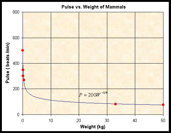
In the allometric section and the computer labs, we saw that many biological applications are reasonably well modeled by a power law relationship. For example, the data from Altman and Dittmer [1] for the pulse, P, as a function of the weight, w, are approximated by the relationship
The pulse is in beats/min, and the weight is in kilograms. Below is a graph of this relationship.

The graph shows an initial steep decrease in the pulse as weight increases, but can one quantify how fast the pulse rate changes as a function of weight? Clearly, for small animals the pulse rate changes more rapidly than for large animals. The derivative of this allometric or power law model provides more details on the rate of change in pulse rate as a function of weight.
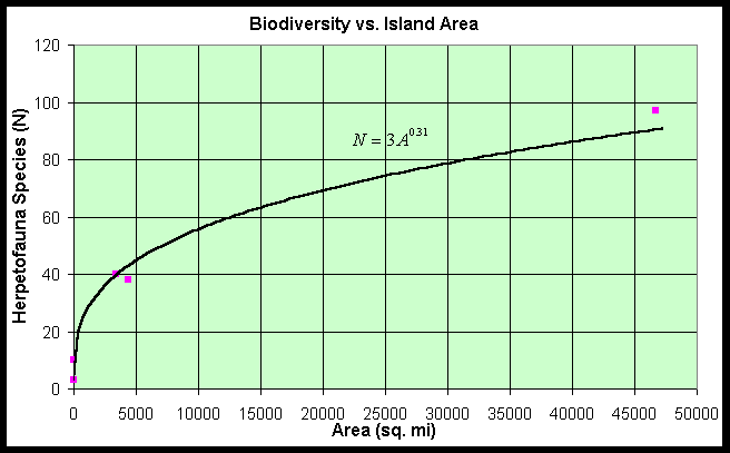
In the computer lab, we saw that the number of species of herpatofauna, N, on Caribbean islands could be related to the area of the island, A, by an allometric model approximated by
A model of this sort is important for obtaining information about biodiversity. A graph of this model is seen below.

Can we use this model to determine the rate of change of numbers of species with respect to a given increase in area? Again the derivative is used to help quantify the rate of change of the dependent variable, N, with respect to the independent variable, A.
We begin with an introduction to some of the notation that we will use. There are several standard notations for the derivative. The two most common are the ones founded by Newton and Leibnitz. For the function f(x), the notation that Leibnitz used was

The Newtonian notation for the derivative is written as follows:
We will use these notations interchangeably, depending on what we are trying to show.
The power rule for differentiation is given by the formula

Examples:
Use the power rule to find the derivatives of the following functions:
|
1. f(x) = x5 |
2. f(x) = x-3 |
|
3. f(x) = x1/3 |
4. f(x) = 1/x4 |
|
5. f(x) = 1/x1/2 |
6. f(x) = 3 |
Solutions:
1. Since n = 5, it follows from the power rule that f '(x) = 5x4.
2. Since n = -3, it follows from the power rule that f '(x) = -3x-4.
3. Since n = 1/3, it follows from the power rule that f '(x) = 1/3x-2/3.
4. Since n = -4, it follows from the power rule that f '(x) = -4x-5.
5. Since n = -1/2, it follows from the power rule that f '(x) = -1/2x-3/2.
6. Since n = 0, the power rule does not apply, but we know that the derivative of a constant is f '(x) = 0.
Examples:
Consider our applications at the beginning of this section. For the model on pulse rate, P = 200w-0.25, we use the power law of differentiation (and the fact that the scalar 200 multiplying the function is uneffected by differentiation) to obtain

The negative sign shows the decrease in the pulse rate with increasing weight. An animal at 16 kg by the allometric model would have a pulse of about 100 (since 200*16-1/4 is 100). The derivative indicates that the pulse rate is decreasing by -50/32 beats/min/kg, so a 17 kg animal should have a pulse rate near 100 - 50/32 = 98 beats/min.
For the biodiversity model, N = 3A1/3, we can differentiate using the power law to obtain
This shows the rate of change of numbers of species with respect to the island area is increasing as the derivative is positive, but the increase gets smaller with increasing island area, since the area has the power -2/3, which puts the area in the denominator of this expression for the derivative.
If a ball is thrown vertically in the air and air resistance is ignored (and we assume that the initial height of the ball is 0), then the height of a ball satisfies the formula,
where v0 is the initial velocity of the ball thrown vertically and g is the acceleration due to gravity. We saw in our previous work that the derivative of this height function is given by the velocity function, which satisfies
This example takes advantage of three rules of differentiation. First, the additive property of derivatives allows consideration of each of the terms in the height function separately. Each of these terms has a scalar multiplier and a power of t. Thus, they use the power rule of differentiation along with a property for scalar multiplication. Below we list the rules for addition and scalar multiplication when taking a derivative.
Other Basic Rules of Differentiation
The operation of differentiation is said to be linear, which means that you can bring out multiplicative constants and the derivative of the sum of two functions is the sum of the derivatives.
Scalar Multiplication Rule:
Assume that k is a constant and f(x) is a differentiable function, then

Additive Rule:
Assume that f(x) and g(x) are differentiable functions, then

Example: Differentiation of polynomials.
Consider the polynomial
From our rules above, it is easy to see that the derivative is
Example:
Clearly other additive powers are handled similarly.
From our rules above, it is easy to see that the derivative is
Worked Examples are available to help with the homework problems.
One of the most commonly used models in population biology is called the logistic growth model. There is a discrete and continuous version of this model, which we will study in some depth later. An earlier section of these notes gave the discrete Malthusian growth model, where the growth of the population is assumed to be proportional to the existing population. The Malthusian growth model is based on unlimited resources. However, as the population increases, the growth rate of most organisms slows to where the population reaches an equilibrium, which is called the carrying capacity of the organism in its environment. The slowing in growth rate can be attributed to a number of factors including crowding (lack of space to reproduce), lack of resources (limited food supply), or build up of waste (toxicity).
The logistic growth function is simply a quadratic function. (Recall that the Malthusian growth function is a linear function.) The basic form of the logistic growth function is

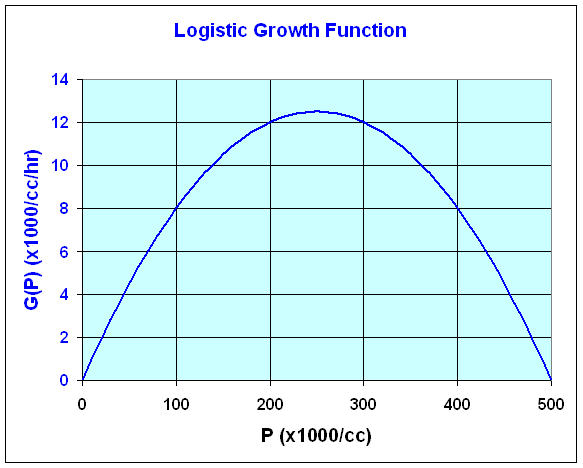
where P is the density of yeast (x1000/cc). Consider the following specific logistic growth function representing the growth of a yeast in a chemostat (a technique often employed for maintaining a yeast culture in breweries). The Malthusian growth rate r = 0.1 (hr-1) (which is about 10% per hour), and the carrying capacity is M = 500 (x1000 yeast/cc). The growth function can be written
G(P) = 0.1P - 0.0002P2.
There are a several interesting points from a biological perspective to study about this growth function. First, when the growth function is zero (no growth) the population is said to be at equilibrium. Biologists (and brewers) frequently want to have their culture growing at peak production rates, which is when the growth function is at its highest point. (Think the maximum height of the ball in the example above.) Let us find these significant points from the growth function above, then create a graph of this function.
The equilibria are found by solving G(P) = 0. We factor the equation above and set it equal to zero
G(P) = 0.1P(1 - 0.002P) = 0.
Thus, either P = 0 (extinction of the population) or 1 - 0.002P = 0, which gives P = 500 (x1000 yeast/cc) (the carrying capacity).
The maximum growth is the vertex of this quadratic function, which is where the derivative is zero. Computing the derivative, we solve
G '(P) = 0.1 - 0.0004P = 0.
Thus, 1 - 0.004P = 0, which gives P = 250. Substituting this value of P into the logistic growth function, we have
G(250) = 0.1(250) - 0.0002(250)2 = 12.5 (x1000 yeast/cc/hr).
Thus, the maximum growth in this culture occurs when the density of yeast in the culture is 250 yeast/cc, and this population of yeast produce 12.5 yeast/cc/hr as the maximum production. Below is a graph of the logistic growth function.

[1] P. L. Altman and D. M. Dittmer, eds. (1964). Biology Data Book. Federation of American Societies for Experimental Biology. pp. 234-235.