1.  Michaelis-Menten Enzyme Kinetics
2. Polynomials and Rational Functions
3. Worked Examples
4. Acid Chemistry Revisited
5. Square Root Function
6. References

The last section introduced quadratic functions and gave the fundamental definitions for a function. This section extends the material from the previous section to other functions. A closer examination of the domains and ranges provide interesting information about the behavior of a function. The graphs of certain functions exhibit asymptotic behavior, such as the saturation effects that are often observed in biological phenomena.

Michaelis-Menten Enzyme Kinetics

Life forms are often characterized by their distinct molecular composition, especially proteins. Proteins are considered the primary building blocks of life. Enzymes are an important class of proteins that catalyze many of the reactions occurring inside the cell. An enzyme has the property of facilitating a biochemical reaction, such that the reaction can occur at biological temperatures. Enzymes are noted for their specificity and speed often under a narrow range of conditions. For example, b-galactosidase catalyzes the break down of lactose into glucose and galactose, then other enzymes further break down these sugars to produce energy for the cell. Urease rapidly converts urea into ammonia and carbon dioxide, very specifically with no other known functions.

The basic mechanism used for simple enzyme reactions, known as the Michaelis-Menten mechanism, has been shown in many experimental situations. The reactants of enzyme reactions, called substrates and denoted by S, are presumed to combine reversibly to the enzyme E to form a enzyme-substrate complex ES. The complex can decompose irreversibly to form a product P and free the enzyme. The reaction can be written as follows:

The law of mass action can be applied to the biochemical equations above to transform them into mathematical equations that describe the kinetics of the molecular reactions. These mathematical equations are known as differential equations, which will be introduced later in the semester. The complete dynamics of the reactions occurring in an enzyme system are often quite complicated, yet may be unnecessary for understanding the basic reaction of the substrate being transformed into the product.

Frequently, it has been observed that the enzyme-substrate complex forms extremely rapidly, while the forward reaction (also known as turnover number), k₂, occurs on a slower time scale. It is assumed that the complex is formed almost instantaneously, a quasi-steady state, then the forward reaction proceeds from there. This assumption gives one of the derivations of the Michaelis-Menten enzyme reaction rate. When a quasi-steady state approximation is made for the initial equilibrium between the free enzyme and substrate and the complex, then the rate of the forward reaction to the product is written as

where [S] is the substrate concentration and V and K_m are kinetic constants determined by the reaction given above. The constant V (also commonly denoted V_max) is called the maximal velocity of the reaction. K_m is the Michaelis constant, and its value is the value of the substrate concentration at which the reaction achieves half of the maximum velocity. This function R is a rational function.

Pate [1] shows that binding of ATP to myosin in forming cross-link bridges to actin for the power stroke of striated muscle tissue satisfies a Michaelis-Menten kinetics. In this particular example, the reaction velocity is an actual velocity of motion, where the chemical energy of ATP is transformed into mechanical energy by movement of the actin filement. The value of K_m gives the concentration of ATP that produces half the maximum velocity of motion for the actin filement. For rabbit psoas muscle tissue, experimental measurements give V_max = 2040 nm/sec and K_m = 150 mM. Below is an applet that shows how the reaction rate R varies as a function of [S] = [ATP] for various values of the maximal velocity V and the Michaelis constant K_m.

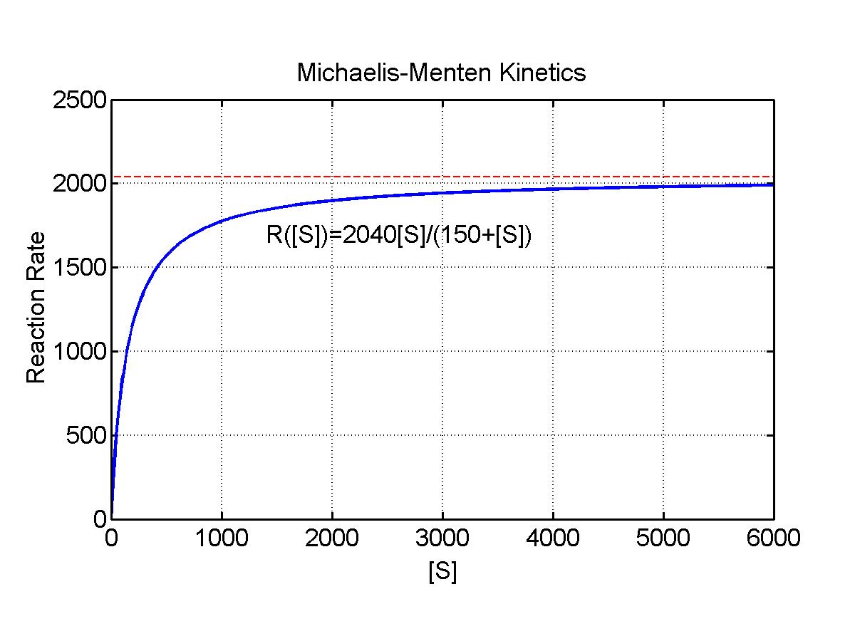
The applet shows typical Michaelis-Menten behavior where the initial rise in the reaction velocity is almost linear, but as the concentration increases, there are diminishing returns with the eventual saturation of the reaction at some maximal rate (the enzymes are working as hard as they can). The Worked Examples section shows how a change of variables allows the conversion of this problem into a linear problem, the Lineweaver-Burk plot.

Polynomials and Rational Functions

One of the most important class of functions, which are commonly studied, are the polynomials. The most general polynomial of order n is written:

where the coefficients a_i are constants and n is a positive integer. In the first section of these notes, we studied linear functions. These are simply first order polynomials. The last section reviewed quadratic functions, which are second order polynomials.

Polynomials are often used in modeling as a means of fitting complicated data. When a polynomial curve fits the data well, then the polynomial, as a function, can be used as a simple model to aid in the interpretation of the data and to construct predictions of how other experiments should behave. There are excellent routines for finding the best least squares fit of a polynomial to data (such as the Excel program that we are frequently using in Lab). Polynomials are defined for all values of x and form very smooth curves. This makes it easy to use them for interpreting data, such as where minimum and maximum values occur or to compute the area under the curve. These phenomena are topics that Calculus covers and will be detailed later in the notes.

As noted above, polynomials are considered nice functions because of their well-behaved properties. Yet even something as basic as finding the roots of an equation (setting p_n(x) = 0) for a polynomial becomes quite difficult for n > 2, and rarely even possible for n > 4. We have the quadratic formula, but few know the formulae for handling third and fourth order polynomials (though they do exist).

Example: Consider the cubic polynomial given by

Find the roots of this equation and graph this cubic polynomial.

Solution: Since we do not have a quadratic formula for cubic equations, we must hope to find a factorization in order to find the roots of the polynomial. In this case, to find the roots, we solve

It follows that the roots of this polynomial are x = 0, -2, or 5. A graph of this cubic polynomial is below with the roots clearly visible as the x-intercepts. Later we will learn (through techniques of Calculus) to find the high point occurring at (-1.08, 6.04) and the low point occurring at (3.08, -30.04).

Polynomials have their limitations, so they are often not appropriate for certain modeling situations. We will need to extend the classes of functions that we study through this course. Our opening example showed Michaelis-Mention kinetics where the reaction rates saturated. This type of behavior is best studied using rational functions.

Rational functions are the quotient of two polynomials. Thus, a function r(x) is a rational function if p(x) and q(x) are polynomials and r(x) = p(x)/q(x). We saw this form of a function in the biochemical analysis of enzyme kinetics given above. The numerator and the denominator were both linear functions, i.e., R([S]) is constructed of the quotient of the linear functions p([S]) = V[S] and q([S]) = K_m + [S].

Since a rational function is a quotient, we have to worry more about the domain of this type of function. If the denominator, q(x), is zero, then the rational function, r(x), becomes undefined at that value of x. Thus, the domain of the rational function, r(x), is all x such that q(x) does not equal zero. The roots of the polynomial q(x) are candidates for vertical asymptotes of r(x). Also, when the order of the polynomial in the numerator of a rational function is less than or equal to the order of the polynomial of the denominator, then a horizontal asymptote occurs.

Asymptotes: Vertical and horizontal asymptotes are very important for determining the shape of a graph.

Vertical Asymptote: When the graph of a function f(x) approaches a vertical line, x = a, as x approaches a, then that line is called a vertical asymptote.

Horizontal Asymptote: When the graph of a function f(x) approaches a horizontal line, y = c, as x becomes very large (either positve or negative), then that line, y = c, is called a horizontal asymptote.

Let r(x) = p(x)/q(x) be a rational function with polynomials p(x) = a_nxⁿ + ... + a₀ of degree n in the numerator and q(x) = b_mx^m + ... + b₀ of degree m in the demoninator.

1. If n < m, then r(x) has a horizontal asymptote of y = 0.
2. If n > m, then r(x) becomes unbounded for large values of x (positve or negative).
3. If n = m, then r(x) has a horizontal asymptote of y = a_n/b_n.

Example: Let us examine the rational function

Find the domain of this function, the x and y-intercepts, and vertical and horizontal asymptotes, then sketch a graph of the function.

Solution: We see that the denominator is zero when x = -2. Thus, the domain of this function must exclude x = -2. Since r(0) = 0 and 10x/(2+x) = 0 implies that x = 0, the x and y-intercepts are easily seen to be zero. Thus, this function passes through the origin.

As x gets very close to -2, the function becomes undefined and the value of r(x) goes to either positive or negative infinity. (See the graph below.) Thus, x = -2 becomes a vertical asymptote. If you consider very large values of x, then the 2 in the denominator becomes insignificant, so the value of r(x) approaches 10x/x = 10. This becomes the horizontal asymptote. The graph below shows r(x) with its vertical and horizontal asymptotes.

A hyperlink is provided to Worked Examples to show you how to work with rational functions.

Acid Chemistry Revisited

In the previous section, weak acids were examined. To find the concentration of the acid, [H⁺], the quadratic formula was needed. The concentration of acid depends on the equilibrium constant and the normality, x, of the weak acid solution. From the previous section, we have

Since the equilibrium constant is fixed depending on the particular weak acid, we see that the [H⁺] is a function of the normality of the solution, x.

We see that this function is neither a polynomial nor a rational function, but the square root function. Below we show a graph of the [H⁺] as a function of x for formic acid, where K_a = 1.77×10^-4. Note that this function has the shape of a quadratic function rotated 90^o.

The pH of the solution is given by -log₁₀([H⁺]), which becomes a composite function. The graph is shown below, but we'll delay studying logarithms until the next section.

Square Root Function

The square root function is the inverse of the quadratic function. It is important to note that the square root function is only defined for positive quantities under the radical. Thus, the domain of a square root function is found by solving the inequality for the function under the radical being greater than zero.

Example: Consider the function

Find the domain of this function and graph the function.

Solution: The domain of this function satisfies x + 2 > 0, so this example has its function defined for x > -2. The graph is shown below.

See the Worked Examples section for more information on square root functions.

References:

[1] E. Pate (1997), "Modeling of muscle crossbridge mechanics," in Case studies in Mathematical Modeling - Ecology, Physiology, and Cell Biology, eds. H. G. Othmer, F. R. Adler, M. A. Lewis, and J. C. Dallon, Prentice-Hall.