Math 121 - Calculus for Biology I
Spring Semester, 2004
Applications of the Derivative - Examples
San Diego State University -- This page last updated 30-Dec-03
|
|
Math 121 - Calculus for Biology I |
|
|---|---|---|
|
|
San Diego State University -- This page last updated 30-Dec-03 |
|
This section provides a series of examples to supplement the lecture section and help with the homework problems. The first examples examine graphing problems. The second example returns to the height of a ball in the air, while the last example uses the derivative to find the maximum and minimum population from a study.
Examples of Graphing Problems: Below are two more examples of graphing problems, where we can apply the derivative and second derivative to help with the sketch of the graph.
Example 1: Use the techniques developed in lecture to find any local or relative minima and maxima and points of inflection for the following polynomial:
Sketch a graph of the function.
Solution: When you want to sketch a graph, the most important part of sketching the graph is finding the extrema (maxima and minima). These are found by finding the derivative and setting it equal to zero. The solutions of the equation for the derivative equal to zero give the critical values, which are substituted back into the the original function. By adding the x and y-intercepts (if possible) and any asymptotes (if they exist) to the sketch, you can get a fairly good idea of what the graph looks like. The second derivative provides nice information to aid with the graph, but it's not nearly as essential in getting a good looking graph.
The y-intercept should always be easy, and in this case, we readily see that (0, 0) is both an x and y-intercept. We can factor this equation and solve for the x-intercept. To find the x-intercept, set y = 0, then factor and solve the equation,
To find the extrema, we take the first derivative of the function and set it equal to zero. Then we solve for xc, where y' = 0.
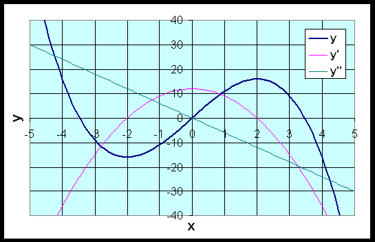
We evaluate the original function at the critical points, giving y(-2) = -16 and y(2) = 16, so the critical points of the function are (-2, -16) and (2, 16). Clearly, the first point is a minimum and the second is a maximum. However, we can check this with the second derivative test. We take the second derivative and evaluate at the critical points to see if they are minima or maxima.
Thus the point (-2, -16) is a local minimum and the point (2, 16) is a local maximum. The points of inflection occur at the point where the second derivative is equal to zero. In this case, the inflection point is at x = 0. This means that the concavity direction changes at point (0, 0). The concavity is upward to the left of (0, 0), and downward to the right of (0, 0). The graph below shows the function and its first and second derivatives.

Example 2: Use the techniques developed in lecture to find the local or relative minima and maxima and points of inflection for the following polynomial:
Sketch a graph of the function.
Solution: See the discussion in Example 1 about the most important steps in sketching a graph. The steps one should always take to create a graph are as follows:
The y-intercept is easily found as (0, 0), which is both an x and y-intercept. We can factor the equation above and solve for the x-intercept
The critical points xc can be found when the first derivative of the function is set equal to zero.
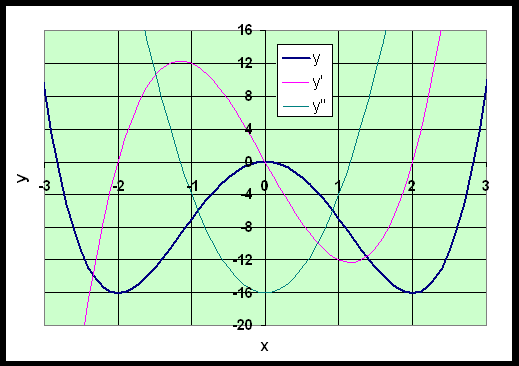
The critical points are at xc = -2, 0, 2. As before, we evaluate the function at each of the critical points, y(-2) = -16, y(0) = 0, and y(2) = -16, so the critical points of the function are (-2, -16), (0, 0), and (2, -16). Clearly, the first point is a minimum, the second is a maximum, and the third is a minimum again.
Again we can check with the second derivative (though usually this step can be omitted because function evaluation gives the relative height of extrema). The nature of these critical points can be found by evaluating the second derivative function at the critical points of the first derivative function. If the result is negative it indicates a maximum and if the result is positive it indicates a minimum.
Thus the critical points indicate local minima at (±2,-16) and a local maximum at (0, 0). The inflection points occur at the zeros of the second derivative function, which are at approximately (±1.155, -8.889). These characteristics are illustrated in the graph below.

Example 3: Height of the Ball Revisited
Consider a ball that is thrown vertically with a initial upward velocity of 64 ft/sec (so v0= 64). The acceleration due to gravity is g = -32 ft/sec2. With these values, the height of the ball satisfies
Find how high this ball travels.
Solution: There are two good ways to solve this problem. From our knowledge of the height function being a quadratic, we could simply find the vertex of the parabola, knowing that it must be at the top of the flight of the ball. Another physical property that can be used to find this maximum for flight of the ball is to recognize that at the top of its flight the ball is temporarily stopped, then its velocity becomes negative as the ball falls back to the ground. Thus, finding the time when the velocity is zero gives the time of the maximum height of the ball.
The velocity function from our differentiation rules is
Solving the velocity equal to zero,
64 - 32 t = 0,
gives the critical time, t = 2 sec. The maximum height of the ball is found by substituing this critical time into the original height equation, so
Example 4: Study of a Population
The ocean water is monitored for fecal contamination by counting certain types of bacteria in a sample of seawater. Over a week where rain occurred early in the week, data were collected on one type of fecal bacteria. The population of the particular bacteria (in thousand/cc), P(t), were best fit by the cubic polynomial
where t is in days.
a. Find the rate of change in population per day, dP/dt. What is the rate of change in the population on the third day?
b. Use the derivative to find when the relative minimum and maximum populations of bacteria occur over the time of the survey. Give the populations at those times. Also determine when the bacterial count is most rapidly increasing.
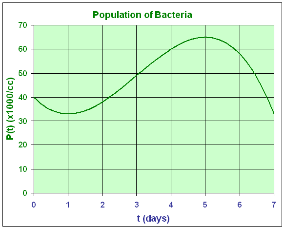
c. Sketch a graph of this polynomial fit to the population of bacteria. When did the rain most likely occur?
Solution: a. To find the rate of change in population per day, we take the derivative of P(t),
![]()
Evaluating this on the third day gives
P '(3) = 12 (x1000/cc/day).
b. The critical points are found by setting the derivative equal to zero. This particular quadratic factors easily, so
P '(t) = -3 t2 + 18 t - 15 = -3(t - 1)(t - 5) = 0.
It follows that the critical values are tc = 1or 5. Substituting the critical values into the population function, we have
Minimum at t = 1 with P(1) = 33 (x1000/cc)
Maximum at t = 5 with P(5) = 65 (x1000/cc).
To find when the population of bacteria is increasing most rapidly, we take the second derivative and set it equal to zero. (Finding the point of inflection.) Thus, we have
P "(t) = -6 t + 18 = -6(t - 3) = 0.
It follows that the population is increasing most rapidly at t = 3 with P(3) = 49 (x1000/cc). Above we see that this maximum increase is
P '(3) = 12 (x1000/cc/day).
c. Below we have the graph of this population. Notice that the population at t = 7 with P(7) = 33 (x1000/cc), which matches the local minimum given above. From the graph, we can guess that the rain fell on the second day of the week with storm runoff polluting the water in the days following.
