![]()
Math 121 - Calculus for Biology I
Spring Semester, 2004
Applications of the Derivative
San Diego State University -- This page last updated 30-Dec-03
|
|
Math 121 - Calculus for Biology I |
|
|---|---|---|
|
|
San Diego State University -- This page last updated 30-Dec-03 |
|
This section examines applications of the derivative to finding maxima and minima. The derivative is valuable for interpreting important aspects of graphs and biological problems. The first problem examines a study of the body temperature of a female during the menstrual cycle and using that to determine fertility. These ideas are generalized to more classical Calculus applications, where the derivative is used to help with sketching the graph of a function.
Body Temperature Fluctuation during the Menstrual Cycle
Mammals are warm-blooded and carefully regulate their body temperature in a narrow range to maintain optimal physiological responses. Variations in body temperature occur during exercise, stress, infection, and other normal situations, but through neurological control, the body self-regulates to maintain a fairly constant temperature. Still there are slight variations including circadian rhythms where each day the body oscillates a few tenths of a degree Celsius (minimum during times of sleep and maximum usually occurring late in the morning). Women also experience a normal body temperature cycle along with their menstrual cycle. Some women monitor their basal body temperature to try to determine their peak period of fertility to maximize (or minimize) the chance of pregnancy. The onset of ovulation often corresponds to the sharpest rise in temperature, which gives peak fertility. (Some claim that by the time a women notices her rise in temperature, she is past her peak fertility, so this type of monitoring is not universally recommended.)
Below is a graph of the basal body temperature taken at the same time each day for a one 28-day period of one woman. The data are fit by a cubic polynomial.
The best cubic polynomial fitting the data above is given by
T(t) = -0.0002762 t3 + 0.01175 t2 - 0.1121 t + 36.41.
From the curve above we want to find the high and low temperatures, then determine the time of peak fertility by finding the time when the temperature is rising most rapidly.
The high and low temperatures occur where the tangent to the curve has a slope of zero. This is where the derivative is zero. From the rules of differentiation, we find the derivative of the temperature.
T '(t) = -0.0008286 t2 + 0.02350 t - 0.1121.
Note that the derivative is a different function from the original function. The roots of this quadratic equation are readily found. They are
t = 6.069 and 22.29 days.
Inserting these values in the original function give
Minimum at t = 6.069 with T(6.069) = 36.1 oC
Maximum at t = 22.29 with T(22.29) = 36.7 oC,
which means that there is only a 0.6 oC difference between the high and low basal body temperature during a 28 day menstrual cycle by the approximating function. The data varied by 0.75 oC.
The day with the maximum increase in temperature is where the derivative is at a maximum. This is the vertex of the quadratic function, T '(t). Clearly, the maximum can be found by the midpoint between the roots of the quadratic equation. However, we can also use the derivative of T '(t) or the second derivative of T(t). The second derivative is given by
T "(t) = -0.0016572 t + 0.02350.
The second derivative is zero at the maximum of T '(t), which occurs at the
Point of Inflection at t = 14.18 with T(14.18) = 36.4 oC.
The maximum rate of change in body temperature is
T '(14.18) = 0.054 oC/day.
This model suggests that the peak fertility occurs on day 14, which is consistent with what is known about ovulation.
See the Worked Examples section for more applications.
Maxima, Minima, and Critical Points
The example above shows that finding when the derivative is zero can give important information about the graph of a function. Another way to view this phenomenon is to examine any graph of a smooth function (which is a function that is continuous and differentiable). It is clear that when you are at a high point of the graph (that is not an endpoint), then the tangent line must be horizontal, which says that the derivative is zero.
Definition: A smooth function f(x) is said to be increasing on an interval (a,b) if f '(x) > 0 for all x in the interval (a,b). Similarly, a smooth function f(x) is said to be decreasing on an interval (a,b) if f '(x) < 0 for all x in the interval (a,b).
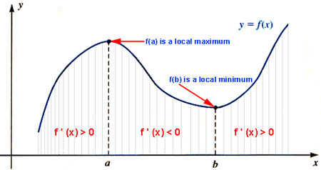
A high point of the graph is where f(x) changes from increasing to decreasing, while a low point on a graph is where f(x) changes from decreasing to increasing. In either case, the derivative passes through zero.
Definition: A smooth function f(x) is said to have a local maximum at a point c, if f '(c) = 0 and f '(x) changes from positive to negative for values of x near c. Similarly, a smooth function f(x) is said to have a local minimum at a point c, if f '(c) = 0 and f '(x) changes from negative to positive for values of x near c.
Clearly, it is important to find where the derivative is zero to find these highest and lowest points on a graph.
Definition: If f(x) is a smooth function with f '(xc) = 0, then xc is said to be a critical point of f(x).
Finding critical points helps find the local high and low points on a graph, but some critical points are neither maxima or minima.
We applied these definitions to a cubic function describing body temperature over a month. Let us examine how finding critical points can help us graph other polynomials. Consider the following examples.
Example: Suppose that
f(x) = x3 - 6x2 - 15x + 2.
Use the information to help sketch a graph of f(x).
Solution: We begin by taking the derivative,
f '(x) = 3x2 - 12x - 15 = 3(x + 1)(x - 5).
The derivative is zero when xc = -1 or 5. Evaluating the function at the critical points, we find f(-1) = 10, which gives a local maximum at (-1,10), and f(5) = -98, which gives a local minimum at (5,-98). The y-intercept is (0,2) another easy point to add to our graph, so we now have good information to make a reasonable sketch of the graph, which is shown below. Note that since this is a cubic equation, the x-intercepts are very hard to find.
The Second Derivative and Concavity
Since the derivative is itself a function, then if it is differentiable, one can take its derivative to find the second derivative often denoted f ''(x). The sign of the second derivative tells where the first derivative is increasing or decreasing. If the first derivative is increasing or the second derivative is positive, then the original function is getting "steeper." The function is said to be concave upward. If the first derivative is decreasing or the second derivative is negative, then the original function is said to be concave downward. Thus, the second derivative is a measure of the concavity of a function. For our smooth functions described above, we can see that maxima generally occur where the function is concave downward, while minima occur where the function is concave upward. This property is often summarized in the following test.
The Second Derivative Test. Let f (x) be a smooth function. Suppose that f '(xc) = 0, so xc is a critical point of f. If f ''(xc) < 0, then xc is a relative maximum. If f ''(xc) > 0, then xc is a relative minimum.
Example: If we return to our example above where f(x) = x3 - 6x2 - 15x + 2, then we see that the second derivative is
The critical points occurred at xc = -1 and 5. Evaluating the second derivative at the critical point xc = -1, we find f ''(-1) = -18, which says the function is concave downward at -1, so this is a relative maximum. Similarly, the second derivative at the critical point xc = 5 is f ''(5) = 18, which says the function is concave upward, so this is a relative minimum.
When the second derivative is zero, then the function is usually changing from concave upward to concave downward or visa versa. This is known as a point of inflection. A point of inflection is where the derivative function has a maximum or minimum, so the function is increasing or decreasing most rapidly. In the application above for the variation of body temperature over one month of a menstrual cycle, the point of inflection represented the potential time of peak fertility by finding where the basal body temperature was increasing most rapidly.
From a graphing perspective, the point of inflection shows the visual change in concavity. It is not nearly as important as extrema, but does provide one more point to aid in graphing the function.
Example: Once again returning to our example above of f(x) = x3 - 6x2 - 15x + 2, where the second derivative is f ''(x) = 6x - 12, we can easily find the point of inflection. We see that f ''(x) = 0 when x = 2. Thus, the point of inflection occurs at (2, -44). This can be see on the graph above.
As usual, for more Worked Examples use this hyperlink.