Computer Lab Help 12

This page is designed to provide helpful information about the laboratory questions. You will find more details in the Lab Manual that accompanies this course. Begin this lab and every lab by introducing yourself to your partner. Determine the times when you can meet together during the week before the lab is due at your next Lab session. You should start this lab and each lab by typing the name of each team member and your computer number on the Lab Cover Page (or a copy of it).

The first WeBWorK problem asks questions about this help page and appropriate lecture material. This should help you work through the Lab more smoothly. This lab explores three problems using differential equations and integrals. The first problem studies how lead builds up in a child, using techniques similar to the ones developed in lecture. The second problem considers a couple of differential equation models used to determine the population growth of a country. The last problem studies how cadium builds in the body over years, and shows how smoking causes increased levels of this toxic compound.

Problem 1 : This problem is very similar to the ones we have recently done in class on Hg in fish or lead in children. This is a variation on the lead in children problem from the Lecture Notes (Differential Equations and Integration) and the homework problems. Mostly, this problem has you showing your expertise in graphing and solving differential equations that you have learned over the semester to date. There are no special instructions needed for this problem (though I might suggest using the Google search engine with key words lead and children to find more information for the last question).

Problem 2: This question uses our least squares techniques from before (Excel's solver). You begin this problem by solving the differential equation using either Maple or techniques from class. Next step up a spreadsheet in Excel with the data on the population from your country in Europe. If Column A contains the year, then you'll want to use Column B for the times after 1950 (i.e., t = 0, 10, 20,...) and Column C will contain the census data. In Column G, you should list your parameters, a, b, and P₀, then place the initial guesses for those parameters in Column H. Good initial guesses for your parameters are to have P₀ be the population in 1950, b = 0.01, and a = 0. You should name these parameters, then in Column D, you insert the formula for the model, which you found earlier, including the named parameters, a, b, and P₀. In column E, you'll put the square error between the data in column C and the model in Column D. Sum the square error, then use Excel's solver to minimize this error and find the best parameters (as you have done before). The remainder of the problem is simply graphing and writing up your results.

Problem 3: The first part of this problem uses our standard methods for solving a linear differential equation. This can be solved either by hand or using Maple. This solution is fit to a data set for cadium building up in the kidney, using our standard least sum of square errors method with Solver in Excel.

The danger of any toxic substance is the exposure to that substance, which is computed by the integral over time of the amount of the toxic substance. You can find the exposure, E(t), by integrating the amount of cadium given by the solution of the differential equation above. This can be done by hand or using Maple. To fit the definite integral starting at t = 0, the arbitrary constant must be set so that E(0) = 0.

The problem asks you to find the exposure for different ages. You can readily evaluate E(t) at those ages by hand or using Maple. We also want to show how the integral can be approximated using the Midpoint and Trapezoid rules. These are readily implemented in Excel (and a downloadable spreadsheet for Numerical Integration is available). The numerical methods are given because the Trapezoid rule can be directly applied to data, which is useful in applications.

Here we describe how to implement the Midpoint, Trapezoid, and Simpson's rules using Excel. The Midpoint rule is particularly easy in Excel. Suppose we want to integrate f(x) from a to b with a stepsize of h = (b - a)/n (n steps). The downloadable spreadsheet considers

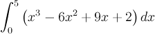
The first Midpoint rule on this spreadsheet divides the interval into 10 even pieces, so h =0.5. With these assumptions we approximate the integral by

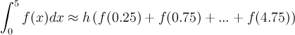
In Excel, create a column starting with a + h/2 (0.25), then add h to each subsequent cell and pull down until you reach b - h/2 (4.75). In the column next to that evaluate f(x) with x values from the first column. The Midpoint rule is simply adding this second column and multiplying by h.

The Trapezoid rule uses a similar techniqe in Excel only the first column starts with a (0), then add h to each subsequent cell and pull down until you reach b (5). Again in the column next to this first column you evaluate f(x) with x values from the first column. The Trapezoid rule for our example with h = 0.5 satisfies:

In this case, we add the first and last cells of the second column, then add 2 times the sum of the rest of the cells and finally multiply by h/2.

The Midpoint and Trapezoid rules give similar estimates to the integral. There is a significantly more accurate numerical integration technique called Simpson's rule. This method is very similar to the Trapezoid rule with slightly different weightings on the elements. There is also the requirement that the interval must be divided into an even number of pieces. For our example, Simpson's rule satisfies:

We see that this numerical integration method is like the Trapezoid rule, except that the middle elements are multiplied in an alternating fashion by 4 and 2 and the entire expression is multiplied by h/3. However, again this is easily implemented in Excel because it is simply adding large columns of numbers with slightly different weights. The downloadable spreadsheet shows how to manage this method in two ways, the first is the tedious clicking on alternating cells and the second is dividing the weighted cells into the ones weighted by 4 and the ones weighted by 2, then using the SUM command.

The last part of the problem shows what happens when someone takes ups smoking. The techniques are the same as above, including actually using the solution from above for the first few years of a person's life before they start smoking. We find the new amount entering the body and solve this new differential equation after the person starts smoking. The exposure now becomes the sum of the exposure before starting smoking plus the years that the person is smoking (assuming a fairly constant annual intake of cigarettes). We simply have two integrals to manage instead of just the one because of the change in habit.