| Joseph M. Mahaffy |
|
| Math 124: Calculus for the Life Sciences | Fall 2016 |
Computer Lab Help 11
This page is designed to provide helpful information about the laboratory questions. You will find more details in the Lab Manual that accompanies this course. Begin this lab and every lab by introducing yourself to your partner. Determine the times when you can meet together during the week before the lab is due at your next Lab session. You should start this lab and each lab by typing the name of each team member and your computer number on the Lab Cover Page (or a copy of it).
The first WeBWorK problem asks questions about this help page and appropriate lecture material. This should help you work through the Lab more smoothly. The first problem studies exponential growth of microbes. This problem explores the power of Malthusian growth when it is unchecked. The second problem examines the differential equations for Malthusian and logistic growth fit to population data for a country. This problem introduces new features of Maple. The last problem studies the time of death of a cat using Newotn's law of cooling and various temperature profiles. This again uses Maple for its solutions.
Problem 1: This problem shows an application related to the Malthusian growth in the differential equations section. The first part of the problem has you calculating volumes and surface areas of different cells, then you use this information with the continuous Malthusian growth model to see how rapidly certain areas and volumes are reached. You are undoubtedly familiar with volumes or surface areas of spheres and cylinders (or can find the formulae on wikipedia); however, one of the cells examined in this lab is ellipsoid in shape. The volume of an ellipsoid has much in common with the volume of a sphere, and you will see that the volume formula is easy to manage. However, the surface area of general ellipsoid can not be found without invoking special functions. Thus, we consider a prolate ellipsoid, which is egg-shaped. It has the closed form solution given in your lab. It does use the inverse trigonometric function, arccos(x). Since cos(x) is not a one-to-one function, the inverse only exists over a limited range of angles. We will only consider what is called the principle arccos(x), which is sometimes denoted Arccos(x) with domain -1 < x < 1 and range 0 < y < p. The function y = arccos(x) gives the angle y whose cosine is x. An example is given by p/3 = arccos(1/2), since cos(p/3) = 1/2. The inverse cosine function is available on all scientific calculators. In Excel, it is written ACOS(x), while in Maple, it is arccos(x).
Finally, you will learn how powerful exponential growth is by trying to analyze Michael Crichton's quote from his book the Andromeda Strain. The hard part of this problem is getting your units correct, so you must be extremely careful when you perform these calculations. This problem can be readily done on a calculator, so it is ideal to do at home! Don't forget that the doubling time and the initial condition (1 cell ) are different from your earlier calculations.
Problem 2: This problem examines the Malthusian and logistic growth models applied to the population of a particular country. (Recall we studied the discrete versions before, so now we want to study the continuous versions.) We use two methods to fit population data to the Malthusian growth model (Excel's Trendline (Exponential fit) and nonlinear least squares fit (similar to before). We also use our nonlinear least squares fit to the logistic growth model. To obtain and appreciate the solutions that we fit for the logistic growth model, we apply a couple of special routines in Maple to better understand the behavior of differential equations.
You will first solve the differential equations using Maple. You can solve many differential equations using Maple's dsolve routine. The Malthusian growth model is used as an example below. The commands to solve this differential equation are simply:
> de := diff(P(t),t)= r*P(t);
# This allows you to view the differential equation.
> dsolve({de, P(0) = P0}, P(t));
# This solves the differential equation with an initial
condition.
> simplify(%); # This
puts the solution in a simpler form.
> p := unapply(rhs(%),t);
# This stores the solution as the function p(t).
Note that you need to be careful using % in Maple as it refers to the last things that you entered, not necessarily the line above (if you are moving your cursor around). You will use the exact solutions to determine matters like the doubling of the population.
The second idea in this problem is called slope fields. Slope fields show at each point on a grid in the time versus population graph the direction of the solution to the differential equation. Thus, a slope pointing in the direction of the derivative (which represents the growth rate or right hand side of the differential equation) is drawn at each point on the grid, which shows the direction the solution proceeds through a particular grid point. Geometrically, the slope field gives the direction of the tangent lines for the solution at each point in the time versus population graph.
For graphing the slope fields, you use the special Maple routine under DEtools with the DEplot routine. Below is an illustration of this command (and its output) for a Newton's Law of Cooling problem
The Maple commands are:
> with(DEtools):
> DEplot(diff(T(t),t)=-0.05*(T(t)-20), T(t),t=0..100, [[T(0)=50],[T(0)=30],[T(0)=5]], T=0..50, color=blue, linecolor=t);
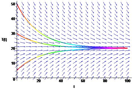
The DEplot command begins with the statement of the differential equation (diff(T(t),t)=-0.05*(T(t)-20)). This is followed by the variable we want to solve (T(t)) and the time interval for the graph (t=0..100). Next the different initial conditions are inserted ([[T(0)=50],[T(0)=30],[T(0)=5]]), which is followed by the range of the dependent variable (T=0..50). I simply added two color options at the end, but this is not necessary.
The slope fields that Maple is drawing are based on the value of the derivative at many points. The slope field points in the direction of the tangent line to the solution curve for the differential equation at each of the points where an arrow is drawn. Closely related to geometric idea is a numerical technique for solving differential equations. You can find a link to details on Euler's Method from the lecture notes for this course (or from Wikipedia on Euler's Method). Simply put, Euler's method uses the definition of the derivative to create a create dynamical model (like we have studied at the beginning of this course). A differential equation of the form:
y ' = f(t,y), y(0) = y0
is approximated by the discrete dynamical model:
yn+1 = yn + h f(tn,yn),
which starts at t0 and y0 and progresses in time steps of h. Thus, tn+1 = tn + h.
Suppose that we have the differential equation with initial condition given by:
y ' = 0.06 y + 0.4 t with y(0) = 5.
This has the solution:
y(t) = (1045 e 0.06t- 1000 - 60 t)/9.
The Euler's formula for this differential equation is given by the simple formula:
yn+1 = yn + h (0.06 yn + 0.4 tn),
This is entered into Excel much like we have done with other discrete dynamical models. There is a hyperlink to an Excel Worksheet for the example above. Suppose that we want to simulate this model with h = 0.5 up until t = 10. In the first column, we enter the time values, so we start with t = 0, then we add h = 0.5 to each cell below that until we reach t = 10. In the second column, we start with y = 0. In the cell below, we use the values from the row above for t and y, so assuming the first values t and y were in A2 and B2, respectively, then in B3, we enter
= B2 + 0.5*(0.06*B2 + 0.4*A2) .
This formula is pulled down to give the Euler simulation. The hyperlinked spreadsheet shows both the Euler simulation and the exact solution, including a graph. Don't forget that often an exact solution is impossible!
Problem 3: Part a of this problem is like the murder problem we worked in class. Parts b and c are modifications that makes the question more realistic by including variable environmental temperatures, but causes certain complications. The solution to this differential equation can be easily found using Maple's dsolve command. The constants k2 and k3 in the solutions appear in a very nonlinear manner in this equation, so it is impossible to solve for k2 and k3 exactly. Thus, you need to use a numerical routine to find the values of k2 and k3. As we have seen often in class before, Maple's fsolve command can be used to solve nonlinear equations. This is done by writing the equation with all the known information at time t = 1. The only unknown is now k2 or k3. In Maple, you write your equation in k2, say f(k2) = 30, where you put in all the information for f(k2). To solve this in Maple, you simply type
fsolve(f(k)=30,k);
and Maple should give you the value of k2. If not, you could have to modify it to say
fsolve(f(k)=30,k=0..10);
Similarly, Maple's fsolve command can be used to find the time of death.
In the Lab Report you are supposed to graph the environmental temperatures (which should be very easy), and you want to graph the temperature of the cat from midnight until 9 AM. While the cat is alive, you graph a horizontal line from midnight to the time of death. Afterwards you use the solution of the differential equation to complete the decaying temperature until 9 AM. Since the solution can be complicated, you might want to copy and paste the solution from Maple to Excel, changing the variable t to the values that you establish for t. This is a good example of graphing piecewise continuous functions in Excel.