| Joseph M. Mahaffy |
|
| Math 124: Calculus for the Life Sciences | Fall 2015 |
Computer Lab Help 13
This page is designed to provide helpful information about the laboratory questions. You will find more details in the Lab Manual that accompanies this course. Begin this lab and every lab by introducing yourself to your partner. Determine the times when you can meet together during the week before the lab is due at your next Lab session. You should start this lab and each lab by typing the name of each team member and your computer number on the Lab Cover Page (or a copy of it).
The first WeBWorK problem asks questions about this help page and appropriate lecture material. This should help you work through the Lab more smoothly. This lab explores three problems using integrals. The first problem studies how cadium builds in the body over years, and shows how smoking causes increased levels of this toxic compound. The second problem models arterial flow of blood using integration. The last problem examines different means of computing averages using integrals and two different approximating functions for a data set of an insect population.
Problem 1: The first part of this problem uses our standard methods for solving a linear differential equation. This can be solved either by hand or using Maple. This solution is fit to a data set for cadium building up in the kidney, using our standard least sum of square errors method with Solver in Excel.
The danger of any toxic substance is the exposure to that substance, which is computed by the integral over time of the amount of the toxic substance. You can find the exposure, E(t), by integrating the amount of cadium given by the solution of the differential equation above. This can be done by hand or using Maple. To fit the definite integral starting at t = 0, the arbitrary constant must be set so that E(0) = 0.
The problem asks you to find the exposure for different ages. You can readily evaluate E(t) at those ages by hand or using Maple. We also want to show how the integral can be approximated using the Midpoint and Trapezoid rules. These are readily implemented in Excel (and a downloadable spreadsheet for Numerical Integration is available). The numerical methods are given because the Trapezoid rule can be directly applied to data, which is useful in applications.
Here we describe how to implement the Midpoint, Trapezoid, and Simpson's rules using Excel. The Midpoint rule is particularly easy in Excel. Suppose we want to integrate f(x) from a to b with a stepsize of h = (b - a)/n (n steps). The downloadable spreadsheet considers
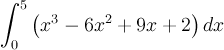
The first Midpoint rule on this spreadsheet divides the interval into 10 even pieces, so h =0.5. With these assumptions we approximate the integral by
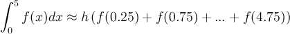
In Excel, create a column starting with a + h/2 (0.25), then add h to each subsequent cell and pull down until you reach b - h/2 (4.75). In the column next to that evaluate f(x) with x values from the first column. The Midpoint rule is simply adding this second column and multiplying by h.
The Trapezoid rule uses a similar techniqe in Excel only the first column starts with a (0), then add h to each subsequent cell and pull down until you reach b (5). Again in the column next to this first column you evaluate f(x) with x values from the first column. The Trapezoid rule for our example with h = 0.5 satisfies:

In this case, we add the first and last cells of the second column, then add 2 times the sum of the rest of the cells and finally multiply by h/2.
The Midpoint and Trapezoid rules give similar estimates to the integral. There is a significantly more accurate numerical integration technique called Simpson's rule. This method is very similar to the Trapezoid rule with slightly different weightings on the elements. There is also the requirement that the interval must be divided into an even number of pieces. For our example, Simpson's rule satisfies:

We see that this numerical integration method is like the Trapezoid rule, except that the middle elements are multiplied in an alternating fashion by 4 and 2 and the entire expression is multiplied by h/3. However, again this is easily implemented in Excel because it is simply adding large columns of numbers with slightly different weights. The downloadable spreadsheet shows how to manage this method in two ways, the first is the tedious clicking on alternating cells and the second is dividing the weighted cells into the ones weighted by 4 and the ones weighted by 2, then using the SUM command.
The last part of the problem shows what happens when someone takes ups smoking. The techniques are the same as above, including actually using the solution from above for the first few years of a person's life before they start smoking. We find the new amount entering the body and solve this new differential equation after the person starts smoking. The exposure now becomes the sum of the exposure before starting smoking plus the years that the person is smoking (assuming a fairly constant annual intake of cigarettes). We simply have two integrals to manage instead of just the one because of the change in habit.
Problem 2: This question begins with a basic maximization problem, which you have done before in Optimization. The second part of this question examines the flow of blood through an artery with conservation of mass. This leads to a definite integral, which is readily solved using the Fundamental Theorem of Calculus. (This can also be computed using Maple.) Most of these calculations can be easily done by hand, but they give important information about the physiology of blood flow in the body. The last part of the question shows what happens to the flow of blood as we consider smaller and smaller arteries. The end of the Help page provides the easy Maple command for solving definite integrals.
Problem 3: This problem uses the material that we are studying in class on definite integrals, which is how the integral finds the area under curves. This is one of the main uses of the integral. It becomes particularly easy if you take advantage of Maple's int command. Part b uses Excel's Trendline with a fourth order polynomial fit, while Part c uses Excel's Solver to find a Fourier fit much like you did in Lab 7, Problem 3 (though a simpler case here). Recall b0 is aproximately the average of the data. We estimate b1 as the difference between the maximum and the average. Assume that tmax > tmin . An estimate for the period is twice the difference between the times for the maximum (tmax) and the minimum (tmin), which gives w approximately p/(tmax - tmin). For the sine function, the phase shift ,f1, is approximately the midpoint of tmin and tmax. For cosine, the phase shift ,f1, is approximately tmax. As a first guess for b2 and f2, take b2 = 70 and f2 = 0. Apply Excel's Solver once, and if any of the parameters are negative, make them positive before applying Solver again. You should apply Solver at least two or three times to be sure that you are at a good point of convergence. You analyze these functions to find the maximum much as you have done before with Maple's diff and fsolve commands. The new part is finding the average using a definite integral, which is basically finding the area under the curve.
To find the area under the curve f(x) from x = a to x = b, you can type the following command in Maple.
int(f(x), x = a..b);
Its that simple! (Clearly, you have to provide an f(x) and the number values of a and b.)
The problem also has you apply the three numerical methods listed above. The downloadable spreadsheet for Numerical Integration and the information above should help you solve this part of the problem.