Example 24.3

A string of length has its ends fixed at , and on an x -axis. The string is under tension, so that when it is given the initial shape , as shown in Figure 24.8 (below), and released, it oscillates. We solve for the motion of the string at any time .

The associated BVP that models the motion of this string is

, t > 0

=

The solution, given by

and

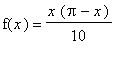
is implemented in Maple as follows. The initial shape function is

> f := x*(Pi-x)/10;

>

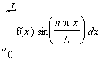
and Figure 24.8 (which shows its graph) is

> plot(f,x=0..Pi,color=black, scaling=constrained, xtickmarks=3, ytickmarks=2, labels=[x,u], labelfont=[TIMES,ITALIC,12]);

>

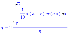
The Fourier coefficients are given by the integral

> q := (2/Pi)*Int(f*sin(n*x),x=0..Pi);

>

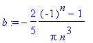
whose value is

> b := simplify(value(q));

>

A peek at the first ten coefficients

> seq(subs(n=k,b),k=1..10);

>

reveals that the odd-indexed terms "survive," the even-indexed terms are zero. Moreover, the coefficients rapidly converge to zero for this function. In fact, they go to zero as , a rapid decrease, as the following conversion to floating point numbers shows.

> seq(evalf(subs(n=k,b)),k=1..10);

>

Hence, a very few terms will be needed to get a good approximation to . We can test this by examining how many terms it takes to get the Fourier series of to approximate well. The first two distinct partial sums in the Fourier series for are

> p1 := sum(b*sin(n*x),n=1..1);
p3 := sum(b*sin(n*x),n=1..3);

>

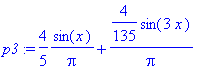
with (thin black) and (thick red) shown in Figure 24.9, below.

> plot([f,p1],x=0..Pi,color=[black,red], thickness=[1,3], scaling=constrained, xtickmarks=3, ytickmarks=2, labels=[x,u], labelfont=[TIMES,ITALIC,12]);

>

This experiment suggests that two terms of the series for might yield a reasonably good approximation, so write

=

that is,

> U := sum(b*sin(n*x)*cos(c*n*t),n=1..3);

>

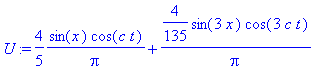
as an approximation to the solution. Set , that is,

> U1 := subs(c=1,U);

>

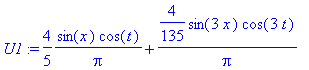
to obtain the graph of the solution surface seen in Figure 24.10, below.

> plot3d(U1, x=0..Pi, t=0..4*Pi, axes=frame, labels=[x,`t `,`u `], labelfont=[TIMES,ITALIC,12], style=hidden, color=red, tickmarks=[3,6,3], orientation=[-45,60]);

>

The plane sections are snapshots in time, freezing the physical motion of the string for each value of . Exhibiting these shapshots in succession forms a movie, or animation, of the physical motion of the string. This animation is given by the following Maple command.

> animate(U1,x=0..Pi,t=0..2*Pi, frames=60, color=black, scaling=constrained, xtickmarks=3, ytickmarks=2, labels=[x,`u `], labelfont=[TIMES,ITALIC,12]);

>

As the string moves in space-time, its history generates a surface, a small part of which we now animate.

>

> F := z -> plot3d(U1, x=0..Pi, t=0..z):
display3d([seq(F(Pi/10*k),k=1..30)],insequence=true, axes=boxed, labels=[x,t,u], labelfont=[TIMES,ITALIC,12], style=hidden, color=red, tickmarks=[3,5,3]);

>