Math 536 -Mathematical Modeling Fall Semester, 2000 Linear Discrete Dynamical Models - Examples
	© 1999, All Rights Reserved, SDSU & Joseph M. Mahaffy San Diego State University -- This page last updated 31-Mar-00

Linear Discrete Dynamical Models - Worked Examples

This section is still under development.

Example 1: For each of the following linear discrete dynamical systems, find the first three iterations, y₁, y₂, and y₃. Also, determine the equilibrium value and determine if it is stable or not.

a. y_n+1 = 1.05 y_n - 200 with y₀= 2000.

b. y_n+1 = 0.6 y_n + 50 with y₀= 100.

Solutions:

a. For y₁, n = 0. Substituting the given value y₀= 2000:

Using the value for y₁ we can find y₂

To find the equilibrium value replace both y_n+1 and y_n with y_e. This is because at equilibrium, all iterations yield exactly the same results.

Thus, y_e = 1.05y_e - 200, or 0.05y_e = 200, and so y_e = 4000. From above, we can see that as n increases, the value of y_n moves away from the equilibrium point, y_e. Note that the value y₀ < y_e, with y_n continually decreasing. The slope of the line is 1.05 on the right hand side, which is greater than 1. This is characteristic of unstable linear discrete dynamical models.

b. For y₁, n = 0. Substituting the given value y₀= 100 :

For the equilibrium, we again let y_e = y_n+1 = y_n, so that y_e = 0.6y_e + 50. Thus, 0.4y = 50, or y = 125. In this case, the solution for y is increasing towards the equilibrium, so that the equilibrium is stable. Note that for this case the slope of the linear model, 0.6, is less than 1, which is characteristic of stable linear discrete dynamical models.
 
 

Example 2: A subject with an unknown lung ailment enters the lab for testing. She is given a supply of air that has an enriched amount of argon gas (Ar). (Recall that atmospheric argon occurs at 0.93% or a concentration of g = 0.0093.) After breathing this supply of enriched gas, two successive breaths are measured with c₁ = 0.0736 and c₂ = 0.0678 of Ar. The model for breathing is given by

Find the fraction of air breathed, q. What is the concentration of argon remaining in her lungs after 5 breaths?

Assume that her tidal volume is measured to be V_i = 220. Find the functional reserve volume, V_r, where q = V_i/(V_i + V_r).

Solution:

Since we are given g and two consecutive values of c_n+1, we can find q as shown below, using

To find the concentration of Ar in her lungs after 5 breaths, we need to know what c₅ is.

To find the functional reserve volume we use the relationship q = V_i/(V_i + V_r).

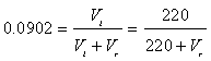
Thus, the tidal volume V_r = 2219.
 
 

Example 3: A population of animals in a particular lake grows according to the Mathusian growth law. In addition, a constant number are entering the lake from a river. Thus, this population satisfies the discrete Malthusian growth model with immigration given by the equation:

where r is the rate of growth and m is the constant number entering the lake. In three successive weeks, the population is measured at P₀ = 500, P₁ = 670, and P₂ = 874. Find the rate of growth r and immigration rate m, then determine the populations expected in the next two weeks.

Solution:

Substituting the given information into the discrete Malthusian growth model gives 2 equations and 2 unknowns (r and m).

Next, we solve for r using substitution for m.

Substituting this value for the rate of growth r back into either equation and solving for the immigration rate m, we find that m = 70. Thus, the model can be rewritten as

With this model we can determine the populations expected in the next two weeks, P₃ and P₄.