Math 122 - Calculus for Biology II Fall Semester, 2004 Optimization - Examples
	© 2000, All Rights Reserved, SDSU & Joseph M. Mahaffy San Diego State University -- This page last updated 29-Jan-04

1. Absolute Extrema of a Polynomial
2. Crop Yield
3. Wire Problem
4. Optimal Production of Pharmaceutical

This section contains more examples of optimization problems. These examples illustrate a range of typical problems.

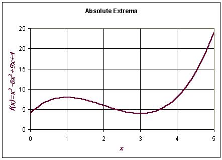
Example 1: Absolute Extrema of a Polynomial

 Consider the cubic polynomial f(x) defined on the interval 0 < x < 5, where

Find the absolute extrema of this polynomial on its domain.

Solution: We begin this problem by finding the derivative of f(x),

Thus, we have critical points at x = 1 and x = 3. To find the absolute extrema, we evaluate f(x) at the critical points and the endpoints of the domain. We obtain:

f(0) = 4 (an absolute minimum),
f(1) = 8 (a relative maximum),
f(3) = 4 (an absolute minimum),
f(5) = 24 (the absolute maximum).

Example 2: Crop Yield

The yield of an agricultural crop depends on the nitrogen in the soil. Crops cannot grow without a source of nitrogen (except many legumes), but if there is too much nitrogen, it becomes toxic and decreases the yield also. Suppose that the yield of a particular agricultural crop satisfies the function

where N is measured in some scaled units. Find the level of nitrogen that produces the maximum crop yield.

Solution: For this function, the domain of interest is N > 0. Again we differentiate the yield function to find the critical points. From the quotient rule, we see that

The critical points are found by solving Y '(N) = 0, which is true when the numerator of the derivative is 0. So the critical points are N = 1 and N = -1. Only the first of these are in the domain with

The endpoints are N = 0 and N tending to infinity. Since Y(0) = 0, it is an absolute minimum. As N tends to infinity, Y(N) decreases toward 0, confirming that we found the absolute maximum. Below shows a graph of this function.
  

Example 3: Wire Problem

A wire length L is cut to make a circle and a square. How should the cut be made to maximize the area enclosed by the two shapes?

Solution: Below is a diagram showing how the wire creates the circle and the square after being cut.

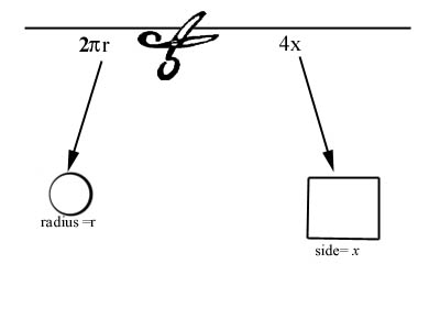
The perimeters of the two figures are constrained to the length of the wire, so

where r is the radius of the circle and x is the length of one side of a square. Notice that the domain is limited by 0 < x < L/4.

The area which is to be maximized is given by the formula

From the constraint, we can solve for r in terms of L and x giving

This is substituted into the formula for the area to form a function depending only on x:

This is differentiated with respect to x. The chain rule is applied to the first term in A(x) and the power rule applies to the second term giving:

To find extrema, we set A'(x) = 0, which is equivalent to

Thus, there is a relative extreme at

If we take the second derivative of A(x), we obtain

Thus, the function is concave upward and the critical point found above is a minimum, not a maximum. (This will be the absolute minimum of this function.) The absolute maximum must be one of the endpoints. Checking at x = 0 and x = L/4, we obtain

The first of these has the smaller denominator, so is the larger. Thus, the maximum occurs when the wire is completely used to create a circle. Geometrically, we know that a circle is the most efficient conversion of a linear measurement into area, so the area produced with the wire completely bent into a circle produces the maximum area. Below shows a graph of the area as a function of x with the left end of the graph corresponding to the wire being completely bent into a circle and the right end corresponding to the wire being bent entirely into a square.

Example 4: Optimal Production of a Pharmaceutical

Bacteria often regulate the production of their proteins based on their rate of growth. Some proteins are produced in higher quantities during high growth rates, while others tend to be produced at a higher rate as the bacteria enter a phase of stress due to limitations in some nutrient source. In the stationary phase, bacteria tend to produce all proteins at a significantly lower rate.

Suppose that the production of a pharmaceutical agent, Q, depends on the population of some bacteria, B, in the following manner:

This function is similar to the Ricker's model that we studied before. When the population of the bacteria is low, then production of the pharmaceutical agent is low as there are not many bacteria producing the pharmaceutical agent. However, when the bacterial population is high, then the effects of stress cause the bacteria to produce other proteins, which again lowers the production of the pharmaceutical agent. There should be an intermediate optimal level of production when there are sufficiently many bacteria producing the agent, yet not enough of them to suppress its production.

The growth of bacteria in culture typically satisfies a logistic growth model (a model that we will later develop). Suppose that the population of bacteria satisfies this growth law and is given by:

Find the time when the production Q is at a maximum.

Solution: The problem asks to find the time when the production of the pharmaceutical agent is at a maximum. However, the production of the pharmaceutical is a function of the population of bacteria, Q(B), (in units of agent), and the population of bacteria is a function of time, B(t) (with time in minutes). Thus, we need to create the composite function Q(B(t)), which is a function that depends on time, t. The production is at its maximum when dQ/dt = 0 (assuming there is a maximum production).

Finding dQ/dt requires the differentiation of a composite function, which uses the chain rule of differentiation. The chain rule for differentiating this composite function gives:

We begin by finding the derivative of Q(B), which uses the product rule and satisfies

(Details of this are left to the reader as it is very similar to the computations for Ricker's model seen in the Product Rule section.) Notice that this has a maximum at B = 500 with Q(500) = 1000 e^-1 = 367.9. Below is a graph of the production of the pharmaceutical agent, Q, as a function of the population of the bacteria, B.

Next we compute the derivative of B(t) = 2000(1 + 99e^-0.01t )^-1. This uses the chain rule twice. By the chain rule we find

We can readily see that this function is always positive or constantly increasing. However, it increases at different rates with varying times. Below is a graph of the population of bacteria, B, as a function of time, t.

These computations make it easy to find dQ/dt, as dQ/dt = Q '(B(t))B '(t) from above. Our calculations above show

For example, if we wanted to know the rate of production att = 0, then first we note that B(0) = 20. We substitute this into the formula above to obtain

Note that Q(B(0)) = 40 e^-0.04 = 38.43 units.

The rate of production at t = 1000 has B(1000) = 2000/(1+ 99e^-10) = 1991 and is given by

Thus, the production is dropping by t = 1000, though the loss is small at this time. Note that Q(B(1000)) = 3982 e^-3.982 = 74.26 units.

So what is the maximum amount of pharmaceutical produced. This will be when dQ/dt = 0. However, this will occur when 1 - 0.002B = 0, as all other terms in the expression for dQ/dt are positive. This implies that B = 500. When we solve B(t) = 500, we find

Thus,

The value of Q(B(100 ln(33))) = 1000 e^-1 = 367.9 units, which is substantially higher than at either t = 0 or t = 1000.

Below is a graph of the composite function, Q(B(t)).