This course is the second semester of the Calculus for Biology sequence at SDSU. The science of Biology is rapidly expanding with an increased need for more quantitative analysis of the data. Thus, mathematics and computers are becoming more important to researchers in Biology. My emphasis for this course will be mathematical modeling of biological systems. (My specialty in research is mathematical biology, so you may find my approach quite different from other math courses that you've seen in the past.) The lecture notes are designed to show how Calculus naturally arises in biological examples from classical and current research. Most sections will begin with a biological model that motivates some aspect of learning Calculus. The example is followed by the mathematical theory required to analyze the biological problem and other related problems. Most sections will include hypertext links to worked examples that will illustrate the types of problems you will encounter in the homework sets. Often additional biological examples are provided after the theoretical section to demonstrate the wide range of applicability of the mathematical techniques.

Biological examples are inherently complex, which complicates the understanding of how mathematical modeling relates to the biological problems. Typical courses in the past use grossly simplified examples, which have resulted in students feeling that Calculus is irrelevant to their study of Biology. My web-based course attempts to use more convincing examples and has a significant portion devoted to computer labs, where technology can aid with the more complicated models. The course is taught with two lectures per week using these web-based notes and one lab period each week where we meet in the computer lab to work on related problems. (I have not found any reasonable texts for teaching this course.) The computer labs will use a mix of computer techniques, which are detailed in the introduction to the lab section. Be sure to review the introductions to the other sections on this website to familiarize yourself with my approach to this course.

Biology is one of the most rapidly expanding and diverse areas in the sciences. The problems encountered in Biology are frequently complex and often not totally understood. Mathematical models provide a means to better understand the processes and unravel some of the complexities. This gives a natural synergistic relationship between the two fields as research expands in the future. The mathematical tools provide ways of developing a better qualitative and quantitative understanding of some biological problems, while the biological problems often stretch the techniques that mathematicians must use to find solutions.

A mathematical model is a representation of a real system. The essence of a good mathematical model is that it is simple in design and exhibits the basic properties of the real system that we are attempting to understand. The model should be testable against empirical data. The comparisons of the model to the real system should ideally lead to improved mathematical models. The model may suggest improved experiments to highlight a particular aspect of the problem, which in turn may improve the collection of data. Thus, modeling itself is an evolutionary process, which continues toward learning more about certain processes rather than finding an absolute reality. This use of mathematics is quite different from K-12 training in mathematics, where mathematics is treated as an absolute with exact answers.

Math 121 is centered about Differential Calculus. One approach for this course is the use of discrete dynamic models to show how growth of a population could could be represented. In the limit as the time interval shrinks for the growth function, the discrete dynamically model becomes a differential equation. For biologists, it is probably easiest to view the derivative as a rate of growth. For students who had a different instructor for Math 121 and did not have much modeling of biological systems, then you will want to read over a collection of topics in my web notes for Math 121 before moving forward with this course. Every effort will be made to review the appropriate material needed to advance with this course, which will concentrate on differential equations, Integral Calculus, and qualitative analysis of systems of differential equations. Topics will also include trigonometric functions.

Example 1: Predator-Prey Model

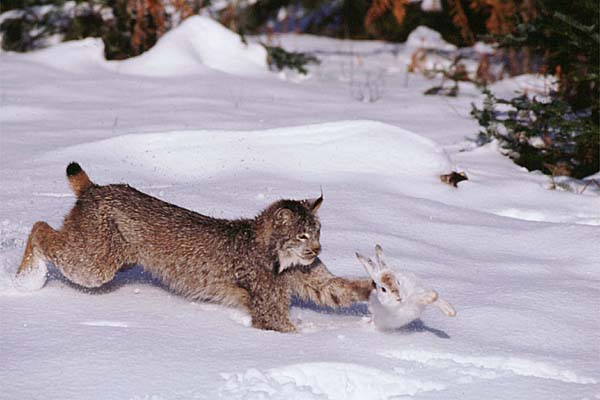
Some of the earliest mathematical models in biology examined population dynamics. Around the turn of the 20^th century, Sir Ronald Ross used mathematical modeling to show that you could drive the disease malaria to extinction without the total eradication of mosquitoes. One of the classic studies of population dynamics was performed by A. J. Lotka [1], who examined the dynamics of predator and prey interactions following the mosquito models first proposed by Ross. It is very difficult to obtain a simple predator-prey interaction because most predators choose from a variety of prey. However, some ecologists examined the records of the Hudson Bay Company and discovered that the pelts of the lynx and hares seemed to oscillate with a fairly regular period. As it happens, the lynx is a very specialized predator that primarily feeds on snowshoe hares. Below is a graph showing data from the Hudson Bay Company for furs from lynx and snowshoe hares.

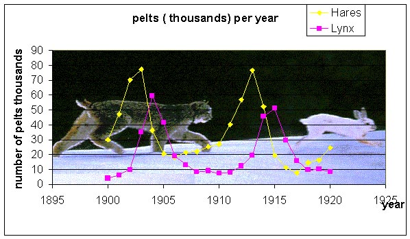
The graph shows a clear correlation between the populations of lynx and hares. First, there is a rapid rise in the population of the hares, which is followed by a rapid rise in the lynx population. Next the hare population plummets, which one or two years later causes the lynx population to fall rapidly. Can this ecological system be explained using a mathematical model? The classic predator-prey model will be analyzed later in the semester.

Example 2: Muscle Contraction

Muscles take chemical energy in our bodies and convert it into motion. How is this accomplished? Skeletal muscle is a striated tissue composed of numerous muscle fibers, which each contain hundreds to thousands of myofibrils. The basic contracting unit of the myofibril is sarcomere, which consists of about 1500 myosin filaments or thick filaments and twice as many actin or thin filaments. These filaments slide past each other during muscular contraction due to cross-bridges between the two filaments. The force of contracting muscles is generated by chemical reactions that cause a conformational strain in the head of the cross-bridges. The figure below shows a single cross-bridge projection coming from the myosin filament and indicates how the motion of the head of this cross-bridge element can pull the actin filament (pictured) toward the center of the cell. The animated gif below shows the cross-bridge cycle that generates this motion.

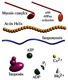
The ratchet theory for muscle contraction was first developed by A. F. Huxley in 1957 [2]. (Huxley won a Nobel prize for his model of the giant axon of the squid, which is seminal work in understanding action potentials in nerves.) The cross-bridge cycle begins with the binding of ATP to the head of the cross-bridge. A calcium ion next binds to this protein, which changes the charges and promotes binding of the cross-bridge to the actin filament. The ATP is hydrolyzed to ADP, which results in a conformational change in the head of the cross-bridge and generates the force to pull the actin filament toward the center of the cell. Next the ADP is released and binding between the filaments is broken, and the cycle is ready to begin anew with the next binding of ATP.

This theory provides the framework for many experiments and refinements that continue today to better understand the precise chemical reactions and forces generated by this process. The process of understanding contraction of a muscle relies on collaborations between biologists studying the muscle tissue, physicists and mathematicians who can calculate the forces generated and required configurations, and chemists who determine key atomic structures, which require massive computational methods. As more detailed molecular studies are performed, you need to know basic principles of Calculus to analyze the data, which is why mathematics is playing an ever increasing role in the study of Biology. You will learn more about contracting muscles in your physiology courses such as Bio 590. A mathematical model for the sliding filament theory is too complicated for this course, but we will be developing some of the basics, such as stretching of an elastic element, which are needed for modeling molecular action of the cross-bridges.
 
 

This course will begin with a review of differentiation by examining some problems in optimization. You should check my webpage for more of this material.

References

[1] A. J. Lotka (1912), Evolution in Discontinuous Systems, Journal of the Washington Academy of Sciences, 2, pp.2, 49, 66

[2] A. F. Huxley (1957), Muscle structure and theories of contraction, Progress in Biophysics 7, 255-318.