1. Falling Cat
2. Differential Equation with Only Time Varying Function
3. Antiderivatives and Integrals
4. Worked Examples
5. Mercury Buildup in Fish in the Great Lakes Region
6. References

This section begins our study of antiderivatives or integrals. We have examined a few differential equations that vary linearly with the unknown function (dependent variable). There have been a variety of applications, including Malthusian growth, radioactive decay, Newton's law of cooling, and contamination of a lake. However, the last section showed that when time varying (the independent variable) terms enter the equation, other techniques are needed. This section looks at differential equations where the object being studied is totally dependent on outside influences, which may be time varying. We will examine objects under the influence of gravity and the time varying buildup of contaminents in an animal.

Falling Cat

The cat has evolved to be a stealthy animal with quick reflexes and extremely good jumping ability. Members of the cat family are considered the best mammalian predators on this planet and occupy an very wide range of niches. Many of the smaller cats have adapted to hunting in trees (or perhaps larger cats have adapted to ground hunting). Thus, they must have tremendous agility. One adaptation that cats have evolved is a very flexible spine, which aids in their ability to spring for prey and absorb shock from their lightning fast strikes. One of the side benefits from this flexible spine is their ability to rapidly rotate their bodies in mid air. With their very sensitive inner ear for balance, which is combined with quick reflexes and a flexible spine, a cat that falls is capable of righting itself very rapidly, insuring that it lands on the ground feet first.

This property of falling feet first has been admired by humans for many years. We are amazed at how few injuries cats have, considering their treacherous lifestyle at heights. It has resulted in jokes about an antigravity device by putting buttered toast on the back of a cat (since buttered toast is believed to always land face down, while cats always land on their feet). Recently, there was a study in the Annals of Improbable Research (1998) on the number of times a particular cat ended up on its feet when dropped from several different heights. There is a serious mathematical research theorem called the Falling Cat Theorem, which examines the torsional behavior of a falling cat in terms of advanced mathematical theory. Other websites relating cats twisting to the physics of skateboards and more detailed physical analysis can be found. In a later section, we will review a scientific study of cats falling out of New York apartments, where paradoxically the cats falling from the highest apartments actually fared better than ones falling from an intermediate height. (Picture and more information can be found from the work of Melvin Leok at Cal Tech.)

Above you can see the dynamics of a cat falling from an inverted position and ending on its feet. It has been shown that a cat can react sufficiently fast that this inversion process (which itself has been the subject of detailed studies) can happen in about 0.3 seconds. With this information, we would like to determine the minimum height from which a cat can be dropped to insure that it lands on its feet.

As noted above, the physics of the cat rotating to get its feet under it during a fall is a moderately complex study in itself. However, our problem is simply to find if the cat has sufficient time to right itself in the air. We are simply going to use Newton's law of motion, which says that mass times acceleration is equal to the sum of all the forces acting on the object. Since the cat is falling only a short distance at a fairly low velocity, it is safe to assume that the only force acting on the cat is gravity. Thus,

where m is the mass of the cat, a is the acceleration of the cat, and -mg is the force of gravity (assuming up is positive), where g is a constant (g = 979 cm/sec² at a latitude like San Diego when you add centripetal acceleration to the standard value given for g, which is 980.7 cm/sec² ).

Recall that acceleration is the derivative of the velocity, and velocity is the derivative of position. If we let h(t) be the height (or position) of the cat at any time t, then the equation above implies that the height of a cat is governed by the differential equation

This is a second order linear differential equation. To find the actual height of the cat at any time after the cat is dropped (or falls off something), this differential equation must be further adjoined by two initial conditions. Since the cat is simply falling, we will assume that the initial velocity starts from rest, so is zero. Thus, v(0) = h'(0) = 0. It is customary to let ground level be a height of zero, so the cat begins at some height above ground level, h(0) = h₀ > 0.

The problem now reduces to solving this initial value problem and finding what values h₀ of produce a solution such that

Since the velocity is the derivative of acceleration, we can begin this problem by finding the velocity at any time. The problem is the first order differential equation given by

Since is -g a constant, we need to find a the velocity function v(t), which upon differentiation produces -g. Thus, we need an antiderivative of a constant. Recall that the derivative of a straight line produces a constant as a straight line is the only function with a constant slope. Thus, we need a straight line with a slope of -g, which in the most general form is

Notice that the antiderivative produces an arbitrary constant, since the derivative of any constant is zero. We use the initial conditions to find the arbitrary constant. Thus,

which gives the velocity for any time as v(t) = -gt. However, the velocity is the derivative of the height, which means we need to repeat this process and find an antiderivative of velocity to determine the height of the cat. To solve the initial value problem

we must find an antiderivative of -gt. We have seen that a quadratic function has a linear derivative, so it is not hard to see that the general solution of this initial value problem becomes

where again c is an arbitrary constant. (You should check this by differentiating and showing it gives the differential equation above.) Again we use the initial condition to give

Thus, the height of the cat any time t for this problem is given by

Using g = 979 cm/sec², we have the equation for height in centimeters as

We evaluate this at t = 0.3 sec and obtain

Thus, the cat must be higher than 44.1 cm for it to have sufficient time to right itself before hitting the ground. (This is about 1.5 feet.)

Differential Equation with Only Time Varying Function

Consider the special class of differential equations where the derivative of the unknown function depends only on a time varying function f(t) (no dependence on y). Thus, the differential equation is given by

The solution to this differential equation is an antiderivative of the function f(t). The antiderivative is also known as the integral. We write the solution of the time varying differential equation as

Antiderivatives and Integrals

A function F(t) is an antiderivative of f(t) if F '(t) = f(t). From the formula for the derivative of tⁿ⁺¹, we see that

so the antiderivative can be written

The integral formula for tⁿ can be written,

Note that the integral formula has an arbitrary constant c, as the derivative of a constant is zero. Since the derivative of a straight line is a constant, the integral of a constant is a linear function. Thus,

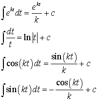
Below is a list of some other basic integrals, which are immediate results from basic formulae for derivatives.

Examples:

We work some examples using these basic integral formulae.

 

More Problems are worked in the Worked Examples section.

Mercury Buildup in Fish in the Great Lakes Region

Fishing is one of the favorite recreational sports for people living around the Great Lakes. However, since the mid-1970s, the Michigan Department of Health has been issuing warnings about eating the fish that are caught from the Great Lakes and some of the surrounding tributaries and inland lakes. The greatest concern for these waterways is the buildup of PCBs in the fatty tissues because of the link of PCBs to cancer and their estrogen effects that appear to be disrupting development in some of the wildlife surrounding these lakes. (It should be noted that health officials report that PCBs have declined 90% since 1975 when they were first monitored.) Another major oncern of health officials is the level of mercury (Hg) that is concentrated in the tissues of the fish that are being eaten by people surrounding the Great Lakes. Mercury, a heavy metal, is a dangerous neurotoxin that is very difficult to remove from the body. It especially concentrates in the tissues of fish, and runs particularly high in the larger predatory fish such as Northern Pike, Lake Trout, Bass, and Walleye. The primary sources of mercury in the Great Lakes region come from the runoff of different minerals that are mined in the region and from incinerators that burn waste, especially batteries that are thrown away (most batteries no longer contain mercury). The mercury problem increases due to some bacteria that convert mercury into the highly soluable methyl mercury, which can enter fish by simply passing over their gills. As the smaller contaminated fish are consumed by larger fish, the mercury becomes more concentrated.

Health officials are particularly concerned about the problems that the higher levels of Hg in the contaminated fish may be causing in children with their developing neural system. Scientists suspect that too much mercury in the diet may lead to impaired development of the nervous system and learning disorders. As a result, there is a warning that young children and pregnant women should limit their consumption to less than one fish per month and especially avoid the larger, fattier, predatory fishes with some fish caught in certain areas to be avoided all together. (For more details on these warnings, the Michigan Department of Health has a webpage on specific problem areas and details on which fish to eat and how to prepare them. Note that the fat problem is for the PCBs, not the Hg.) Others are recommended to limit their comsumption to less than one fish a week and avoid eating the larger fish, such as Lake Trout over 22 inches.

So why do fish build up the dangerous levels of Hg in their tissues? One important reason is that Hg is not easily removed from the system, so once it is ingested, it tends to remain in the body. (The best way to remove heavy metals is the use of chelating agents.) Mathematically, this build up is seen by the integral of the ingested Hg over the lifetime of the fish. Thus, we would expect that the older and larger fish should have more Hg than the younger fish. Below we present a model for the build up of Hg in a Lake Trout living in some lake in the Great Lakes region. (There is not a warning for mercury in the Great Lakes surrounding Michigan, but there is a general advisory about mercury in all inland lakes.)

In the homework problems for the Linear Differential Equations section, Problem 13 gives the von Bertalanffy equation for the growth of a fish. A similar model could be used to describe the weight, w(t), of a Lake Trout. The record for a Lake Trout in Michigan is 27.9 kg (124 cm in length). Assume that the weight of a Lake Trout satisfies the differential equation:

We can use our techniques from the Linear Differential Equations section to solve this equation, obtaining the solution:

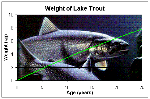
We can see that this solution levels off at a 25 kg Lake Trout. It takes 5.5 years for these fish to reach 2 kg and about 15 years to reach 5 kg. A graph of the weight of Lake Trout with age is shown below.

 

A fish will eat a quantity of food that is roughly proportional to its weight. Let H(t) be the amount of Hg (in mg) in a growing Lake Trout. By assuming that the concentration of Hg in its food is constant (though in fact, the larger fish will eat more heavily contaminated, larger fish), then the rate of Hg that is added to the tissues of a fish in the Great Lakes will satisfy the differential

where k = 0.03 mg/yr. With this information and using the information above, H(t) is found by integrating the right hand side of the equation above. This gives

 

The two integrals fit the formulae above, so we take the antiderivatives, and the solution becomes:

 

The initial condition gives H(0) = 0, so it follows that

Thus, the solution giving the amount of mercury in a growing Lake Trout is

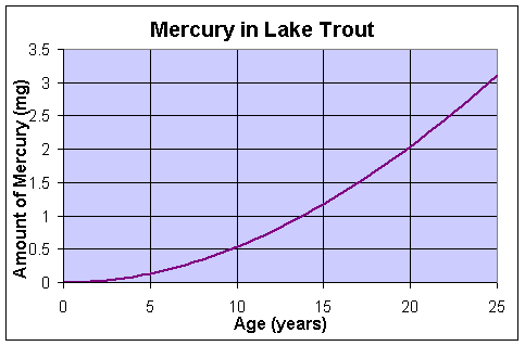
A graph of the total amount of mercury in a Lake Trout (in mg) as a function of age (in years) is given below.

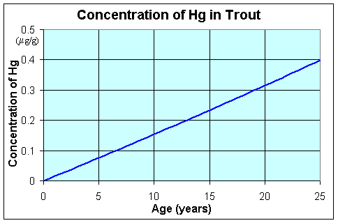
This shows that the amount of mercury in an aging Lake Trout increases substantially as it eats more and more prey containing mercury. However, it is more important to know what the concentration of mercury in the flesh of the Lake Trout that is eaten (as you generally eat the same amount of fish). Below shows a graph of the concentration of mercury in a Lake Trout as it ages. It becomes clear why the Michigan Department of Health advises against eating larger, hence older and more mercury containing fish. The concentration of Hg is measured in mgrams (of mercury) per gram (of fish), and is given by

References:

[1] Jared M. Diamond (1988), Why cats have nine lives, Nature 332, pp 586-7.