|
|
Math 122 - Calculus for Biology II |
|
|---|---|---|
|
|
San Diego State University -- This page last updated 26-Aug-01 |
|
|
|
Math 122 - Calculus for Biology II |
|
|---|---|---|
|
|
San Diego State University -- This page last updated 26-Aug-01 |
|
This section continues the development of some ecological models for two species that are competing for the same resources. As we did in the previous section, an equilibrium analysis is performed. The analysis is extended to provide a geometric understanding of equilibria. Nullclines are introduced, which will allow easier qualitative analysis of 2-Dimensional differential equations.
Chemostat with Two Yeast Populations
One method for maintaining a culture of yeast used in brewing beer is to create a chemostat. A chemostat is a large vat, where nutrients are pumped into the vat at a constant rate, then the growing culture is removed at the same rate. Under ideal conditions, a monoculture of yeast grows according to the logistic growth equation, and soon a constant supply of uniform concentration of the yeast flows from the chemostat. This allows the brewmaster a consistent supply of the yeast culture, which guarantees a uniform product with the desired characteristics. Unfortunately, it is almost impossible to keep a consistent monoculture of the yeast. The vat often gets infected with a competing yeast or bacteria that destroys the uniformity and lowers the quality of the beer.
In this section, we want to study what happens when two species compete for a single resource. One of the classical studies in this area comes from the book Struggle for Existence by G. F. Gause [1]. His experiments did not use an actual chemostat, but rather changed the nutrient in a closed vessel regularly (every 3 hours), which is similar to a chemostat. He performed a number of experiments to test competition of microbial species. One set of experiments examined the standard brewers yeast, Saccharomyces cerevisiae, and a slower growing yeast, Schizosaccharomyces kephir. He tested these organisms in cultures by themselves to find their growth parameters using a logistic growth model, then he mixed the cultures to determine how the organisms reacted when they competed in the same nutrient medium. He notes that though he used a standard medium, he was not certain of all the concentrations of the different components in the medium, which complicates the ecological model since the species could be utilizing different components of the medium. However, we will assume that their is probably some limiting nutrient for which these two species compete. The logistic growth model for S. cerevisiae was studied in more detail in the special section on solving the logistic growth model, while the logistic growth model for S. kephir was given as an exercise in the homework.
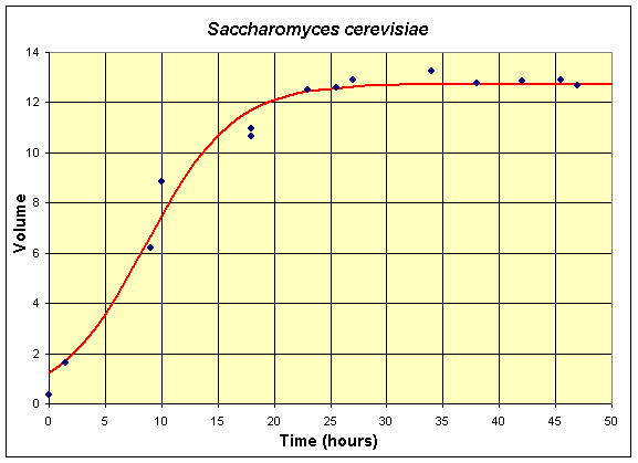
Below we present a series of tables and graphs of the two yeast species competing in the Gause experiments. We also give the best solutions to the single species data using the logistic growth model. The first table and graph combines two experiments of Gause using only S. cerevisiae in the culture. These data are shifted by 6 hours from the original experiment because no data were collected until 6 hours from innoculation of the yeast culture.
Table for Single Species Culture of Saccharomyces cerevisiae
|
Time (hr) |
0
|
1.5
|
9
|
10
|
18
|
18
|
23
|
25.5
|
27
|
34
|
38
|
42
|
45.5
|
47
|
|
Volume |
0.37
|
1.63
|
6.2
|
8.87
|
10.66
|
10.97
|
12.5
|
12.6
|
12.9
|
13.27
|
12.77
|
12.87
|
12.9
|
12.7
|
The graph shows the best fitting solution to the data, and its formula is given below.

If we let X(t) be the population for S. cerevisiae, then the differential equation for this yeast population that best fits these data is given by

which has the solution (see Logistic Growth section)
![]()
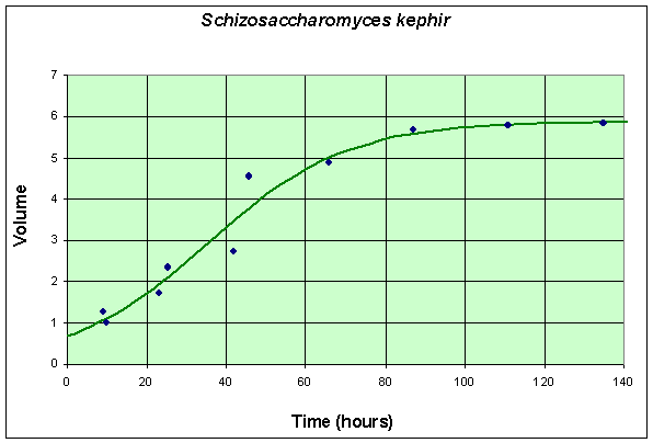
The second table and graph combines two experiments of Gause using only S. kephir in the culture. To match with the data for the experiment with S. cerevisiae, these data are also shifted by 6 hours from the original (which had the first measurement at 15 hours after innoculation). These data are collected over a much longer time period because of the slow growing nature of S. kephir.
Table for Single Species Culture of Schizosaccharomyces kephir
|
Time (hr) |
9
|
10
|
23
|
25.5
|
42
|
45.5
|
66
|
87
|
111
|
135
|
|
Volume |
1.27
|
1.0
|
1.7
|
2.33
|
2.73
|
4.56
|
4.87
|
5.67
|
5.8
|
5.83
|
The graph shows the best fitting solution to the data, and its formula is given below.

If we let Y(t) be the population for S. kephir, then the differential equation for this yeast population that best fits these data is given by

which has the solution (see Logistic Growth section)
![]()
Finally, we present a table that shows the competition of S. cerevisiae and the slower growing S. kephir that Gause performed in two experiments. Once again the data are shifted by 6 hours from the original experiment to match the first time when data was actually collected after innoculation of the yeast cultures.
Table for Mixed Species Culture of Saccharomyces cerevisiae and Schizosaccharomyces kephir
|
Time (hr) |
0
|
1.5
|
9
|
10
|
18
|
18
|
23
|
25.5
|
27
|
38
|
42
|
45.5
|
47
|
|
Volume (S. cerevisiae) |
0.375
|
0.92
|
3.08
|
3.99
|
4.69
|
5.78
|
6.15
|
9.91
|
9.47
|
10.57
|
7.27
|
9.88
|
8.3
|
| Volume (S. kephir) |
0.29
|
0.37
|
0.63
|
0.98
|
1.47
|
1.22
|
1.46
|
1.11
|
1.225
|
1.1
|
1.71
|
0.96
|
1.84
|
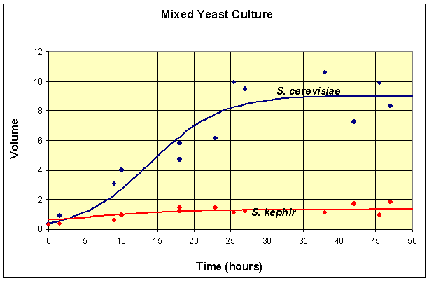
We need a model that finds the populations of these two species competing for the limiting resources. The single species models provide some information on the parameters in the model, but this mixed population experiment adds complications to the mathematical model, which are developed below. A graph of the data and the best fitting solution to a competition model is shown after the development of the model.
Let us create a mathematical model for two competing species. Let X(t) be one species of yeast and Y(t) be a second species of competing yeast. In the absence of the second species of yeast, we would expect X(t) to satisfy a logistic growth model. Thus, the dynamics for its growth is given by the equation:
The first term, a1X(t), is the standard Malthusian growth, and the second term, -a2X2(t), is the loss due to crowding. It is also known as intraspecies competition. In the Gause experiments listed above, the single species experiments for S. cerevisiae allowed us to find the parameters a1 and a2.
However, we are assuming that there is competition from a second species, interspecies competition. This is modeled very much like the loss term in the predator-prey model. Thus, to the logistic model given above, we need to add the interspecies competition term, -a3X(t)Y(t), so the equation for the dynamics of the first species of yeast is given by
Simlarly, the growth of the second species of yeast satisfies the differential equation
![]()
Again, the Gause experiments for the single species experiments for S. kephir allowed us to find the parameters b1 and b2. It remains to find the parameters for the interspecies competition, a3 and b3.
The two differential equations above create a system that describes the dynamics of two competing species of yeast. So what does this system of differential equations suggest for possible outcomes for these two competing species of yeast? This system of differential equations cannot be solved exactly, so we need to resort to our techniques of qualitative analysis along with some numerical methods to find the remaining parameters.
As we have seen before, the equilibria are found by setting the derivatives equal to zero. Thus, we need to solve the system of nonlinear equations

for the equilibria Xe and Ye. The solution to this system of nonlinear equations is given by
and
Ye = 0 or b2Ye + b3Xe = b1.
Algebraically, if Xe = 0, then either Ye = 0 or Ye = b1/b2. The symmetry of the relations show that when Ye = 0, then there is another equilibrium at Xe = a1/a2. These three equilibria all have extinction of at least one of the species. There is one other equilibrium solution that allows coexistence of both species, which results from solving simultaneously the equations a2Xe + a3Ye = a1 and b2Ye + b3Xe = b1. The result is the fourth (coexistence) equilibrium

For the Gause experiment with the two yeast species S. cerevisiae and S. kephir, the data seem to indicate a coexistence of the the two species with a leveling off of the populations (though not as clearly as in the single species experiments). Estimates of the value for this coexistence equilibrium provide an initial guess that allows us to perform a least squares best fit to the data using techniques that are developed in the numerical methods section for two differential equations. The system of differential equations for the mixed populations of yeast are simulated using an Improved Euler's method with the parameters, a3 and b3, and the initial populations X(0) and Y(0) allowed to vary. This simulation is minimized using a least squares best fit to the data. (More details and a link to an Excel spreadsheet are provided in the Numerical Solutions for 2-D Differential Equations.) The resulting system of differential equations with the best fitting initial conditions is given by

A graph of the data and the solutions to these differential equations is shown below.

This simulation shows that at t = 50, the model for the population of S. cerevisiae is at X(50) = 8.97 and the model population of S. kephir is at Y(50) = 1.35.
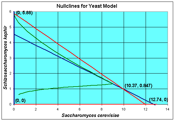
From our discussion above, this system of differential equations has the four equilibria given by
Xe = 0 and Ye = 0
Xe = 0 and Ye = 5.880
Xe = 12.74 and Ye = 0
Xe = 10.37 and Ye = 0.8469
Thus, at t = 50, the simulation of the model has not gone to any of these equilibria, but is closest to the coexistence equilibrium. In fact, the maximum population of S. cerevisiae is reached at t = 44 with X(44) = 8.98, then this population begins declining. By t = 500, the population of S. cerevisiae is X(500) = 0.01, while the population of S. kephir is Y(500) = 5.83. So it follows that over very long periods of time, S. kephir will drive S. cerevisiae to extinction. This process is known as competitve exclusion and is the most frequent outcome of two competing species. Despite the fact that S. kephir grows more slowly, it has an inherent competitve advantage over S. cerevisiae and dominates given sufficient time.
A geometric method for finding the equilibria and extending our understanding of the solutions of the differential equations is to find the nullcines of the differential equations. The definition of a nullcline is simply when the derivative is equal to zero, which is what the equations above show. Graphically, we draw the nullclines in the XY-plane. Below we show a graph for our competition model of yeast with the nullcines and the solution in the phase space.

[1] G. F. Gause, Struggle for Existence, Hafner, New York, 1934.