Natural oscillations have been observed between the populations of predators and their prey. The predator-prey model was developed independently in the 1920s by Alfred J. Lotka and Vito Volterra. This problem examines the Lotka-Volterra model with data on lynx and snowshoe hares from North Canada. Between 1845 and 1935, the Hudson Bay company kept good records on the numbers of animals trapped in Canada [1], which should reflect their relative populations. Below is a table on the lynx and snowshoe hare pelts collected between 1900 and 1920 (with Excel data sheet).
|
Year |
Hares (x1000) |
Lynx(x1000) |
Year |
Hares (x1000) |
Lynx (x1000) |
|
1900 |
30 |
4 |
1911 |
40.3 |
8 |
|
1901 |
47.2 |
6.1 |
1912 |
57 |
12.3 |
|
1902 |
70.2 |
9.8 |
1913 |
76.6 |
19.5 |
|
1903 |
77.4 |
35.2 |
1914 |
52.3 |
45.7 |
|
1904 |
36.3 |
59.4 |
1915 |
19.5 |
51.1 |
|
1905 |
20.6 |
41.7 |
1916 |
11.2 |
29.7 |
|
1906 |
18.1 |
19 |
1917 |
7.6 |
15.8 |
|
1907 |
21.4 |
13 |
1918 |
14.6 |
9.7 |
|
1908 |
22 |
8.3 |
1919 |
16.2 |
10.1 |
|
1909 |
25.4 |
9.1 |
1920 |
24.7 |
8.6 |
|
1910 |
27.1 |
7.4 |
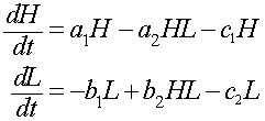
The predator-prey model for the lynx L(t)
and hares H(t)
is given by the following system of differential equations:

a. Give a brief description of the growth and death terms in the differential equations above for the lynx L(t) and hares H(t), explaining what the mathematical terms mean ecologically. Find the average number lynx and hares for the data above.
b. We need to find the best parameters in the model above, a1, a2, b1, b2, H0, and L0. Euler's method for this model is given by:

Let h = 0.1, then use the Euler's method above to simulate the model and compare to the data. Apply Excel's Solver to find the least squares best fit to the parameters. List the least squares best fit to the data giving both the values for the parameters and the sum of squares error.
c. Graph both the data and Euler simulation for both populations. Use the simulation to estimate the length of period for oscillations of this predator-prey interaction. The solution to the differential equation is periodic, so give an explanation why the simulation is not periodic. Find the percent error between the model and the data for the years 1903, 1909, 1914, and 1919. From your simulation, determine the year and value of the minimum and the maximum for this approximation.
d. With the parameters found above, find all equilibria for this model.
e. Suppose that an extensive trapping effort removes 10% of each population. The model becomes

where c1 = c2 = 0.1. Find the new equilibria for this model and compare it to the equilibria found in Part d.
[1] E. P. Odum (1953), Fundamentals of Ecology, Philadelphia, W. B. Saunders.